Christoﬀel functions with power type weights

(1)

Christoffel functions with power type weights

^∗

Tivadar Danka^† Vilmos Totik^‡ December 20, 2018

Abstract

Precise asymptotics for Christoffel functions are established for power type weights on unions of Jordan curves and arcs. The asymptotics involve the equilibrium measure of the support of the measure.

The result at the endpoints of arc components is obtained from the corresponding asymptotics for internal points with respect to a different power weight. On curve components the asymptotic formula is proved via a sharp form of Hilbert’s lemniscate theorem while taking polynomial inverse images. The situation is completely different on the arc components, where the local asymptotics is obtained via a discretization of the equilibrium measure with respect to the zeros of an associated Bessel function. The proofs are potential theoretical, and fast decreasing polynomials play an essential role in them.

1 Introduction

Christoffel functions have been the subject of many papers, see e.g. [12], [13], [18], and the extended reference lists there. They are intimately connected with orthogonal polynomials, reproducing kernels, spectral properties of Jacobi matrices, convergence of orthogonal expansion and even to random matrices, see [5], [13] and [18] for their various connections and applications.

The possible applications are growing, for example recently a new domain recovery technique has been devised that use the asymptotic behavior of Christoffel functions, see [6]; and in the last 4-5 years several important methods for proving universality in random matrix theory were based on them, see [1], [8], [9] and [10]. The aim of the present paper is to complete, to a certain extent, the investigations concerning their asymptotic behavior on Jordan curves and arcs.

Let µ be a finite Borel measure on the plane such that its support is compact and consists of infinitely many points. The Christoffel functions

(3)

associated withµare defined as

λ_n(µ, z₀) = inf

Pn(z0)=1

Z

|P_n|²dµ, (1.1)

where the infimum is taken for all polynomials of degree at mostnthat take the value 1 at z. If p_k(z) = p_k(µ, z) denote the orthonormal polynomials with respect toµ, i.e. Z

p_np_mdµ=δ_n,m, thenλ_ncan be expressed as

λ⁻¹_n (µ, z) = Xn

k=0

|p_k(z)|².

In other words,λ⁻¹(µ, z) is the diagonal of the reproducing kernel K_n(z, w) =

Xn

k=0

p_k(z)p_k(w)

which makes it an essential tool in many problems. It is easy to see that, with this reproducing kernel, the infimum in (1.1) is attained (only) for

P_n(z) = K_n(z, z₀) K_n(z₀, z₀), see e.g. [20, Theorem 3.1.3]).

The earliest asymptotics for Christoffel functions for measures on the unit circle or on [−1,1] go back to Szeg˝o, see [21, Th. I’, p. 461]. He gave their behavior outside the support of the measure, and for some special cases he also found their behavior at points of (−1,1). The first result for a Jordan arc (a circular arc) was given in [4]. By now the asymptotic behavior of Christoffel functions for measures defined on unions of Jordan curves and arcs Γ is well understood: under certain assumptions we have for points z∈Γ that are different from the endpoints of the arc components of Γ

n→∞lim nλ_n(µ, z₀) = w(z₀)

ωΓ(z0), (1.2)

where w is the density of µ with respect to the arc measure s_Γ on Γ, and ω_Γ is the density of the equilibrium measure (see below) with respect tos_Γ. For the most general results see [22] and [24].

What is left, is to decide the asymptotic behavior at the endpoints of the arc components. It turns out that this problem is closely related to the asymptotic behavior away from the endpoints, but for measures of the form dµ(x) =|z−z₀|^αds_Γ(z),α >−1, and the aim of this paper is to find these

(4)

asymptotic behaviors. When µ is of the just specified form, then we shall show (for the exact formulation see the next section),

n→∞lim n^1+αλ_n(µ, z₀) = 1

(πω_Γ(z₀))^α+12^α+1Γα+ 1 2

Γα+ 3 2

(1.3)

whenz₀ is not the endpoint of an arc component of Γ, while at an endpoint

n→∞lim n^2α+2λn(µ, z0) = Γ(α+ 1)Γ(α+ 2) (πM(Γ, z₀))^2α+2 , whereM(Γ, z₀) is the limit ofp

|z−z₀|ω_Γ(z) asz→z₀ along Γ.

This paper uses some basic notions and results from potential theory.

See [2], [3], [16] or [19] for all the concepts we use and for the basic theory.

In particular,ν_Γ will denote the equilibrium measure of the compact set Γ.

Since the asymptotics reflect the support of the measure, in all such questions a global condition, stating that the measure is not too small on any part of Γ, is needed (for example, ifµis zero on any arc of Γ, then (1.3) does not hold any more). This global condition is the regularity condition from [19]: we say that µ, with support Γ, belongs to theReg class if

sup

Pn

kP_nkΓ

kPnkL²(µ)

!1/n

→1

as n → ∞, where the supremum is taken for all polynomials of degree at mostn, and wherekP_nkΓ denotes the supremum norm on Γ. The condition says that in then-th root sense theL^∞(µ) andL²(µ)-norms are almost the same. The assumption µ ∈ Reg is a very weak condition – see [19] for several reformulations as well as conditions on the measure µ that implies µ ∈ Reg. For example, if Γ consists of rectifiable Jordan curves and arcs with arc measures_Γ, then any measure dµ(z) =w(z)ds_Γ(z) withw(z) >0 s_Γ-almost everywhere is regular in this sense.

Actually, it is not even needed that the support Γ of the measure µ be a system of Jordan curves or arcs, the main theorem below holds for any Γ that is a finite union of continua (connected compact sets). However, it is needed thatz₀ lies on a smooth arc J of the outer boundary of Γ: the outer boundary of Γ is the boundary of the unbounded connected component of C\Γ. It is known that the equilibrium measure ν_Γ lives on the outer boundary, and ifJ is a smooth (sayC¹-smooth) arc on the outer boundary, then on J the equilibrium measure is absolutely continuous with respect to the arc measure s_J on J: dν_Γ(z) = ω_Γ(z)ds_J(z). We call this ω_Γ the equilibrium density of Γ.

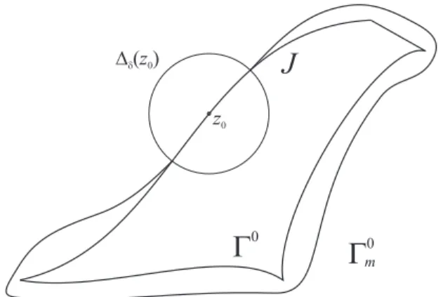
The following theorem describes the asymptotics of the Christoffel function at points that are different from the endpoints of the arc-components/parts of Γ, see Figure 1 for illustration.

(5)

G

z₀

Figure 1: A typical position where Theorem 1.1 can be applied Theorem 1.1 Let the support Γ of a measure µ ∈ Reg consist of finitely many continua, and let z₀ lie on the outer boundary of Γ. Assume that the intersection ofΓwith a neighborhood of z₀ is a C²-smooth arcJ which con- tainsz₀in its (one-dimensional) interior. Assume also that in this neighbor- hooddµ(z) =w(z)|z−z₀|^αds_J(z), where w is a strictly positive continuous function and α >−1. Then

n→∞lim n^1+αλn(µ, z0) = w(z0)

(πω_Γ(z₀))^α+12^α+1Γα+ 1 2

Γα+ 3 2

. (1.4) The second main theorem of this work is about the behavior of the Christoffel function at an endpoint, see Figure 2. Ifz₀ is an endpoint of a smooth arcJ on the outer boundary of Γ, then atz₀ the equilibrium density has a 1/p

|z−z0|behavior (see the proof of Theorem 1.2), and we set M(Γ, z0) := lim

z→z0, z∈Γ

p|z−z0|ω_Γ(z). (1.5)

Theorem 1.2 Let Γ and µbe as in Theorem 1.1, but now assume that the intersection of Γ with a neighborhood of z0 is a C²-smooth Jordan arc J with one endpoint atz₀. Then

n→∞lim n^2α+2λ_n(µ, z₀) = w(z₀)

(πM(Γ, z0))^2α+2Γ(α+ 1)Γ(α+ 2). (1.6) These results can be used, in particular, if the measure is supported on a finite union of intervals on the real line, in which case the quantitiesω_Γ(x) and M(Γ, x) have a rather explicit form. Let Γ = ∪^kj=0⁰ [a_2j, a_2j+1] with disjoint [a_2j, a_2j+1]. Then the equilibrium density of Γ is (see e.g. [23, (40),

(6)

G

z₀

Figure 2: A typical position where Theorem 1.2 can be applied (41)] or [19, Lemma 4.4.1])

ω_Γ(x) =

Qk0−1

j=0 |x−λ_j| πqQ2k0+1

j=0 |x−aj|

, x∈Int(Γ), (1.7)

whereλj are the solutions of the system of equations Z a_2k+2

a2k+1

Qk0−1

j=0 (t−λ_j) qQ2k0+1

j=0 |t−a_j|

dt= 0, k= 0, . . . k0−1. (1.8)

It can be easily shown that these λ_j’s are uniquely determined and there is one λj on every contiguous interval (a2j+1, a2j+2). Now if a is one of the endpoints of the intervals of Γ, saya=a_j₀, then

M(Γ, a) =

Qk0−1

j=0 |a−λ_j| πqQ2k0

j=1, j6=j0|a−aj|

. (1.9)

This whole work is dedicated to proving Theorem 1.1 and Theorem 1.2.

Actually, the latter will be a relatively easy consequence of the former one, so the main emphasis will be to prove Theorem 1.1. The main line of reasoning will be the following. We start from some known facts for simple measures like |x|^αdx on the real line, and get some elementary results for a model case on the unit circle via a transformation. Then we prove from these simple cases that Theorem 1.1 is true for lemniscate sets, i.e. level sets of polynomials. This part will use the polynomial mapping in question to transform the already known result to the given lemniscate. Then we prove

(7)

the theorem for finite unions of Jordan curves. Recall that a Jordan curve is a homeomorhic image of a circle, while a Jordan arc is a homeomorhic image of a segment. From the point of view of finding the asymptotics of Christoffel functions there is a big difference between arcs and curves: Jordan curves have interior and can be exhausted by lemniscates, so the polynomial inverse image method of [23] is applicable for them, while for Jordan arcs that method cannot be applied. Still, the pure Jordan curve case is used when we go over to a Γ which may have arc components, namely it is used in the lower estimate. The upper estimate is the most difficult part of the proof; there Bessel functions enter the picture, and a discretization technique is developed where the discretization of the equilibrium measure of Γ is done using the zeros of appropriate Bessel functions combined with another discretization based on uniform distribution. Once the case of Jordan curves and arcs have been settled, the proof of Theorem 1.1 will easily follow by approximating a general Γ by a family of Jordan curves and arcs.

2 Tools

In what follows,k · kK denotes the supremum norm on a setK, and s_Γ the arc measure on Γ (when Γ consists of smooth Jordan arcs or curves).

We shall rely on some basic notions and facts from logarithmic potential theory. See the books [2], [3], [16] or [17] for detailed discussion.

We shall often use the trivial fact that if µ, ν are two Borel measures, then µ ≤ ν implies λn(µ, x) ≤ λn(ν, x) for all x. It is also trivial that λ_n(µ, z)≤µ(C) (just use the identically 1 polynomial as a test function in the definition ofλ_n(µ, z)).

Another frequently used fact is the following: if{n_k}is a subsequence of the natural numbers such that n_k+1/n_k →1 ask→ ∞, then for anyκ >0

lim inf

n→∞ n^κλn(µ, x) = lim inf

k→∞ n^κ_kλn_k(µ, x), (2.1) and

lim sup

n→∞ n^κλ_n(µ, x) = lim sup

k→∞

n^κ_kλ_n_k(µ, x). (2.2) In fact, sinceλ_n(µ, x) is a monotone decreasing function of n, forn_k≤n≤ n_k+1 we have

n n_k+1

κ

n^κ_k+1λn_k+1(µ, x)≤n^κλn(µ, x)≤ n

n_k κ

n^κ_kλn_k(µ, x), and both claims follow because n/n_k and n/n_k+1 tend to 1 as n (or n_k) tends to infinity.

(8)

2.1 Fast decreasing polynomials

The following lemmas on the existence of fast decreasing polynomials will be a constant tool in the proofs.

Proposition 2.1 Let K be a compact subset on C, Ω the unbounded com- plement of C\K and let z₀ ∈ ∂Ω. Suppose that there is a disk in Ω that contains z₀ on its boundary. Then, for every γ > 1, there are constants c_γ, C_γ, and for every n ∈ N polynomials S_n,z₀_,K of degree at most n such thatS_n,z₀_,K(z₀) = 1, |S_n,z₀_,K(z)| ≤1 for all z∈K and

|Sn,z0,K(z)| ≤Cγe^−nc^γ^|z−z⁰^|^γ, z∈K. (2.3) For details, see [22, Theorem 4.1]. This theorem will often be used in the following form.

Corollary 2.2 With the assumptions of Proposition 2.1 for every 0< τ <

1, there exists constants c_τ, C_τ, τ₀ > 0 and for every n ∈ N a polynomial S_n,z₀_,K of degree o(n) such that S_n,z₀_,K(z₀) = 1, |S_n,z₀_,K(z)| ≤ 1 for all z∈K, and

|S_n,z₀_,K(z)| ≤C_τe^−c^τⁿ^τ⁰, |z−z₀| ≥n^−τ. (2.4) Proof. Let 0< εbe sufficiently small and select γ >1 so that 1−ε−τ γ >

0. Lemma 2.1 tells us that there is a polynomial P_n with deg(P_n) ≤n^1−ε such that

|P_n(z)| ≤C_γe^−c^γⁿ^{1−(ε+τ γ)}, |z−z₀| ≥n^−τ, and this proves the claim withSn,z0,K =Pn.

There is a version of Lemma 2.1 where the decrease is not exponentially small, but starts much earlier than in Lemma 2.1.

Proposition 2.3 Let K be as in Proposition 2.1. Then, for every β < 1, there are constants c_β, C_β >0, and for everyn= 1,2, . . . polynomials P_n of degree at most n such thatP_n(z₀) = 1,|P_n(z)| ≤1 for z∈K and

|Pn(z)| ≤C_βe^−c^β^(n|z−z⁰^|)^β, z∈K. (2.5) See [25, Lemma 4].

It will be convenient to use these results when n > 1 is not necessarily integer (formally one has to take the integral part of n, but the estimates will hold with possibly smaller constants in the exponents).

(9)

2.2 Polynomial inequalities

We shall also need some inequalities for polynomials that are used several times in the rest of the paper.

We start with a Bernstein-type inequality.

Lemma 2.4 Let J be a C² closed Jordan arc and J₁ a closed subarc of J not having common endpoint with J. Then, for every D > 0, there is a constant C_D, such that

|P_n^′(z)| ≤C_DnkP_nkJ, dist(z, J₁)≤D/n, holds for any polynomialsP_n of degree n= 1,2, . . ..

See [22, Corollary 7.4].

Next, we continue with a Markov-type inequality.

Lemma 2.5 LetK be a continuum. IfQnis a polynomial of degree at most n= 1,2, . . ., then

kQ^′_nkK ≤ e

2cap(K)n²kQ_nkK, (2.6) where cap(K) denotes the logarithmic capacity of K.

In particular, if K has diameter 1, then

kQ^′_nk^K ≤2en²kQnk^K. (2.7) For (2.6) see [15, Theorem 1], and for the last statement note that ifK has diameter 1, then its capacity is at least 1/4 ([16, Theorem 5.3.2(a)]).

Next, we prove a Remez-type inequality.

Lemma 2.6 Let Γbe a C¹ Jordan curve or arc, and assume that for every n= 1,2, . . ., Jn is a subarc of Γ, and J_n^∗ is a subset of Jn such that

s_Γ(J_n\J_n^∗) =o(n⁻²)s_Γ(J_n),

where s_Γ denotes the arc-length measure on Γ. Then, for any sequence {Q_n}of polynomials of degree at most n= 1,2, . . ., we have

kQ_nkJn = (1 +o(1))kQ_nkJ_n^∗. (2.8) Proof. It is clear from theC¹ property that sΓ(Jn)∼diam(Jn) uniformly inJ_n (meaning that the ratio of the two sides lies in between two positive constants).

Make a linear transformation z → Cz such that, after this transformation, the arc ˜J_n that we obtain from J_n has diameter 1. Under this transformationJ_n^∗ goes into a subset ˜J_n^∗ of ˜J_n for which

s_J_˜

n( ˜J_n\J˜_n^∗) =o(n⁻²)s_J_˜

n( ˜J_n), (2.9)

(10)

and Q_n changes into a polynomial ˜Q_n of degree at most n. (2.8) is clearly equivalent to its˜-version.

Let M =kQ˜_nkJ˜n. By Lemma 2.5, the absolute value of ˜Q^′_n is bounded on ˜J_nby 2en²M, hence ifz, w∈J˜_n, then

|Q˜_n(z)−Q˜_n(w)| ≤2en²M s_J_˜

n(zw), (2.10)

where zw is the arc of ˜J_n lying in between z and w. By the assumption (2.9) for everyz∈J˜_nthere is aw∈J˜_n^∗ with

s_J_˜

n(zw) =o(n⁻²)s_J_˜

n( ˜J_n) =o(n⁻²) because s_J_˜

n( ˜J_n)∼diam( ˜J_n) = 1. Choose herez ∈J˜_n such that |Q˜_n(z)|= M. Since |Q˜n(w)| ≤ kQ˜nkJ^˜_n^∗, we get from (2.10)

M =|Q˜_n(z)| ≤ kQ˜_nkJ˜_n^∗+o(1)M, and the claim follows.

We shall frequently use the following, so called Nikolskii-type inequalities for power type weights. In it we write that a Jordan arc isC¹⁺-smooth if there is aθ >0 such that the arc in question isC^1+θ-smooth.

Lemma 2.7 Let J be a C¹⁺-smooth Jordan arc and letJ^∗⊂J be a subarc of J which has no common endpoint with J. Let z0 ∈ J be a fixed point, and for α > −1 define the measure ν_α on J by dν_α(u) = |u−z₀|^αds_J(u).

Then there is a constantC depending only onα, J andJ^∗ such that for any polynomials Pn of degree at most n= 1,2, . . . we have

kP_nkJ^∗ ≤Cn^(1+α)/2kP_nkL²(να), (2.11) if α≥0, and

kP_nkJ^∗ ≤Cn^1/2kP_nkL²(να), (2.12) if −1< α <0.

The same is true if dν_α(u) = w(u)|u−z₀|^αds_J(u) with some strictly positive and continuous w.

Proof. In view of [26, Lemmas 3.8 and Corollary 3.9] (use also that ν_α is a doubling weight in the sense of [26]) uniformly inz∈J^∗ we have for large nthe relation

λ_n(ν_α, z)∼ν_α(l_1/n(z)),

(11)

whereA∼B means that the ratio lies in between two constants, and where l_1/n(z) is the arc of J consisting of those points of z that lie of distance

≤1/n fromz. Ifα≥0, then

να(l_1/n(z))≥ c n^1+α, while for −1< α <0

ν_α(l_1/n(z))≥ c n,

with some positive constantcwhich depends only onα, JandJ^∗. Therefore, we have for allz∈J^∗ the inequality

λ_n(ν_α, z)≥ c

n^1+α (2.13)

ifα≥0 and

λ_n(ν_α, z)≥ c

n (2.14)

when−1< α <0.

For example, (2.13) means that ifα≥0 and|P_n(z)|= 1 for somez∈J^∗, then necessarily

n^1+α c

Z

J|Pn|²dνα≥1,

which is equivalent to saying that for anyP_n andz∈J^∗ n^1+α

c Z

J|P_n|²dν_α≥ |P_n(z)|²,

and this is (2.11). In a similar manner, (2.12) follows from (2.14).

It is clear that this proof does not change if ν_α is as in the last sentence of the lemma.

Lemma 2.8 If α > −1, then there is a constant C_α such that for any polynomialP_n of degree at most n the inequality

kPnk[−1,1]≤Cαn^(1+α^∗^)/2 Z 1

−1|Pn(x)|²|x|^αdx ^1/2

(2.15) holds withα^∗= max(1, α).

Proof. We follow the preceding proof, but now bothJ and J^∗ agree with [−1,1].

LetJ =J^∗ = [−1,1],z0 = 0, ∆n(z) = 1/n² ifz∈[−1,−1 + 1/n²] orz∈ [1−1/n²,1], and set ∆_n(z) =√

1−z²/nifz∈[−1 + 1/n²,1−1/n²]. If now l_1/n(z) is the interval [z−∆_n(z), z+∆_n(z)] intersected with [−1,1], then [26,

(12)

Lemmas 3.8 and Corollary 3.9] state that fordν_α(x) =|x−z₀|^αdx=|x|^αdx on [−1,1] we have

λ_n(ν_α, z)∼ν_α(l_1/n(z)).

Ifα≥0, then

να(l_1/n(z))≥cmin 1

n², 1 n^1+α

, while for −1< α <0

ν_α(l_1/n(z))≥ c n², with some positive constant c. Hence,

λ_n(ν_α, z)≥ c n² if−1< α≤1, while

λn(να, z)≥ c n^1+α ifα≥1, from which (2.15) follows exactly as before.

The Nikolskii inequalties can be combined with the following estimate to get an upper bound for the extremal polynomials that produceλ_n(µ, z).

Lemma 2.9 With the assumptions of Theorem 1.1 we have λn(µ, z0)≤Cn^−(α+1)

with some constantC that is independent of n.

Proof. Just use the polynomials P_n from Proposition 2.3 with β = 1/2 and K = Γ. Let δ > 0 be so small that in the δ-neighborhood of z0 we have the dµ(z) = w(z)|z−z₀|^αds_Γ(z) representation for µ. Outside this δ-neighborhood|S_n,z₀_,Γ|is smaller thanC_βexp(−c_β(nδ)^1/2), so

Z

|Sn,z0,Γ|²dµ≤C Z

e^−2c^β^(n|t|)^1/2|t|^αdt+Ce^−2c^β^(nδ)^1/2 ≤Cn^−α−1, which proves the claim.

We close this section with the classical Bernstein-Walsh lemma, see [27, p. 77].

Lemma 2.10 Let K⊂Cbe a compact subset of positive logarithmic capacity, letΩbe the unbounded component ofC\K, and g_Ω the Green’s function of this unbounded component with pole at infinity. Then, for polynomialsP_n of degree at most n= 1,2, . . ., we have for any z∈C

|P_n(z)| ≤e^ng^Ω^(z)kP_nkK.

(13)

3 The model cases

3.1 Measures on the real line

Our first goal is to establish asymptotics for the Christoffel function at 0 with respect to the measure dµ(x) = |x|^αdx, x ∈ [−1,1]. We do this by transforming some previously known results.

In what follows, for simpler notations, if dµ(x) =w(x)dx, then we shall write λn(w(x), z) for λn(µ, z).

Proposition 3.1 Forα >−1 we have

n→∞lim n^2α+2λ_n

|x|^α

[0,1],0

= Γ(α+ 1)Γ(α+ 2). (3.1) Proof. It follows from [10, (1.10)] or [9, Theorem 4.1] that

n→∞lim n^2α+2λ_n

(1−x)^α

[−1,1],1

= 2^α+1Γ(α+ 1)Γ(α+ 2), (3.2) from which the claim is an immediate consequence if we apply the linear transformationx→(1−x)/2.

Proposition 3.2 Forα >−1 we have

n→∞lim n^α+1λ_n

|x|^α

[−1,1],0

=L_α, (3.3)

where

L_α:= 2^α+1Γα+ 1 2

Γα+ 3 2

. (3.4)

Proof. Let us agree that in this proof, whenever we write Pn, Rn etc. for polynomials, then it is understood that the degree is at mostn.

We use that (for continuousf) Z 1

0

f(x)|x|^αdx= Z 1

−1

f(x²)|x|^2α+1dx. (3.5) Assume first thatP_2nis extremal forλ_2n

|x|^α

[−1,1],0

, i.e. P_2n(0) = 1

and Z 1

−1|P_2n(x)|²|x|^αdx=λ_2n

|x|^α

[−1,1],0

. Define

R_2n(x) = P_2n(x) +P_2n(−x)

2 .

(14)

Then R_2n(0) = 1, and R_2n is a polynomial in x², hence R_2n(x) = R^∗_n(x²) with some polynomialR^∗_n, for which R^∗_n(0) = 1 and deg(R^∗_n)≤n. Now we have

Z 1

−1|R_2n(x)|²|x|^αdx= Z 1

−1|R^∗_n(x²)|²|x|^αdx = Z 1

0 |R^∗_n(x)|²|x|^α−1² dx

≥ λn

|x|^α−1²

[0,1],0

. With the Cauchy-Schwarz inequality and with the symmetry of the measure

|x|^αdx, we have Z 1

−1|R_2n(x)|²|x|^αdx≤ 1 4

Z 1

−1

|P_2n(x)|²+ 2|P_2n(x)||P_2n(−x)|+|P_2n(−x)|²

|x|^αdx

≤ 1 2

Z ₁

−1|P_2n(x)|²|x|^αdx +1

2 Z 1

−1|P2n(x)|²|x|^αdx

!1/2 Z 1

−1|P2n(−x)|²|x|^αdx

!1/2

= Z 1

−1|P_2n(x)|²|x|^αdx=λ_2n

|x|^α

[−1,1],0

. Combining these two estimates, we obtain

λ_n

|x|^α−1²

[0,1],0

≤λ_2n

|x|^α

[−1,1],0

. On the other hand, if now P_n is extremal for λ_n

|x|^α−1²

[0,1],0

, then λ_n

|x|^α−1²

[0,1],0

= Z 1

0 |P_n(x)|²|x|^α−1² dx = Z 1

−1|P_n(x²)|²|x|^αdx

≥ λ_2n

|x|^α

[−1,1],0

, therefore we actually have the equality

λ_n

|x|^α−1²

[0,1],0

=λ_2n

|x|^α

[−1,1],0

, (3.6)

from which the claim follows via Proposition 3.1 (see also (2.1) and (2.2) withn_k= 2k).

Note also that this proves also that if P_n(x) is the n-degree extremal polynomials for the measure |x|^α−1²

[0,1], then P_n(x²) is the 2n-degree extremal polynomial for the measure|x|^α

[−1,1].

(15)

3.2 Measures on the unit circle

LetµT be the measure on the unit circleT defined bydµT(e^it) =wT(e^it)dt, where

wT(e^it) = |e^2it+ 1|^α 2^α

|e^2it−1|

2 , t∈[−π, π). (3.7) We shall prove

n→∞lim n^α+1λ_n(µT, e^iπ/2) = 2^α+1L_α (3.8) where L_α is from (3.4), by transforming the measure µT into a measure µ_[−1,1]supported on the interval [−1,1] and comparing the Christoffel functions for them. With the transformatione^it→cost, we have

Z π

−π

f(cost)wT(e^it)dt= 2 Z 1

−1

f(x)w_[−1,1](x)dx, where

w_[−1,1](x) =|x|^α. Setdµ_[−1,1](x) =w_[−1,1](x)dx.

LetPn be the extremal polynomial for λn(µ_[−1,1],0) and define Sn(e^it) =Pn(cost) 1 +e^i(t−π/2)

2

!⌊ηn⌋

e^in(t−π/2),

whereη >0 is arbitrary. This S_n is a polynomial of degree 2n+⌊ηn⌋ with Sn(e^iπ/2) = 1. For any fixed 0< δ <1

Z π/2+δ

π/2−δ |S_n(e^it)|²wT(e^it)dt≤

Z π/2+δ

π/2−δ |P_n(cost)|²wT(e^it)dt

≤ Z 1

−1|P_n(x)|²w_[−1,1](x)dx

=λ_n(µ_[−1,1],0).

(3.9)

To estimate the corresponding integral over the intervals [−π, π/2−δ] and [π/2 +δ, π], notice that

t∈[−π,π]\[π/2−δ,π/2+δ]max

1 +e^i(t−π/2) 2

⌊ηn⌋

=O(qⁿ) (3.10) for someq <1. From Lemma 2.8 we obtain

kP_nk[−1,1]≤Cn^1+|α|/2kP_nkL²(µ_[−1,1])≤Cn^1+|α|/2, and so

Z π/2−δ

−π

+ Z π

π/2+δ

!

|S_n(e^it)|²wT(e^it)dt=O(n^1+|α|/2qⁿ) =o(n^−α−1).

(16)

Therefore, using thisS_n as a test polynomial forλ_deg(S_n₎(µT, e^iπ/2) we conclude

λ_deg(S_n₎(µT, e^iπ/2)≤λ_n(µ_[−1,1],0) +o(n^−α−1), and so

lim sup

n→∞ 2n+⌊ηn⌋α+1

λ_2n+⌊ηn⌋(µT, e^iπ/2)≤lim sup

n→∞ 2 +⌊ηn⌋/nα+1

n^α+1λn(µ_[−1,1],0)

= (2 +η)^α+1Lα, where we used Proposition 3.2 for the measureµ_[−1,1].

Since η >0 was arbitrary, lim sup

n→∞

n^α+1λ_n(µT, e^iπ/2)≤2^α+1L_α (3.11) follows (see also (2.2)).

Now to prove the matching lower estimate, let S_2n(e^it) be the extremal polynomial forλ_2n(µT, e^iπ/2). Define

P_n^∗(eît) =S2n(eît) 1 +eî(t−π/2) 2

!2⌊ηn⌋

e−(n+⌊ηn⌋)i(t−π/2)

and Pn(cost) =P_n^∗(e^it) +P_n^∗(e^−it). Note that Pn(cost) is a polynomial in cost of deg(P_n)≤n+⌊ηn⌋ and P_n(0) = 1. With it we have

λ_deg(P_n₎(µ_[−1,1],0)≤ Z 1

−1|P_n(x)|²w_[−1,1](x)dx= 1 2

Z π

−π|P_n(cost)|²wT(e^it)dt.

(3.12) First, we claim that for every fixed 0< δ <1

|P_n(cost)|²=|P_n^∗(e^it)|²+O(qⁿ), t∈[π/2−δ, π/2 +δ],

|P_n(cost)|²=|P_n^∗(e^−it)|²+O(qⁿ), t∈[−π/2−δ,−π/2 +δ],

|P_n(cost)|²=O(qⁿ) otherwise,

(3.13)

hold for someq <1. Indeed,

|P_n(cost)|² =|P_n^∗(eît)+P_n^∗(e^−it)|² ≤ |P_n^∗(eît)|²+2|P_n^∗(eît)||P_n^∗(e^−it)|+|P_n^∗(e^−it)|². If we apply Lemma 2.7 to two subarcs (say of length 5π/4) ofTthat contain the upper, resp. the lower half of the unit circle, then we obtain that

kP_n^∗k^T≤ kS_2nk^T ≤Cn^(1+|α|)/2kS_2nkL²(µ_T)≤Cn^(1+|α|)/2. Therefore (use (3.10))

|P_n^∗(e^it)| ≤Cqⁿn^(1+|α|)/2, t∈[−π, π]\[π/2−δ, π/2 +δ].

(17)

These imply (3.13).

Now we have Z π

−π|Pn(cost)|²wT(e^it)dt=

Z π/2+δ π/2−δ

+

Z −π/2+δ

−π/2−δ

!

|Pn(cost)|²wT(e^it)dt +

Z −π/2−δ

−π

+

Z π/2−δ

−π/2+δ

+ Z π

π/2+δ

!

|Pn(cost)|²wT(e^it)dt.

(3.13) tells us that the last three terms areO(qⁿ). For the other two terms we have, again by (3.13),

Z π/2+δ

π/2−δ |P_n(cost)|²wT(e^it)dt=

Z π/2+δ

π/2−δ |P_n^∗(e^it)|²wT(e^it)dt+O(qⁿ)

≤

Z π/2+δ

π/2−δ |S_2n(e^it)|²wT(e^it)dt+O(qⁿ)

≤λ_2n(µT, e^iπ/2) +O(qⁿ) and similarly,

Z −π/2+δ

−π/2−δ |P_n(cost)|²wT(e^it)dt≤λ_2n(µT, e^iπ/2) +O(qⁿ).

Combining these estimates with (3.12), we can conclude λ_deg(P_n₎(µ_[−1,1],0)≤λ2n(µT, e^iπ/2) +O(qⁿ), therefore

lim inf

n→∞ deg(P_n)^α+1λ_deg(P_n₎(µ_[−1,1],0)≤lim inf

n→∞ (n+⌊ηn⌋)^α+1 λ_2n(µT, e^iπ/2) +O(qⁿ)

≤lim inf

n→∞ (1 +⌊ηn⌋/n)^α+1 1

2^α+1(2n)^α+1λ_2n(µT, e^iπ/2).

From this, in view of Proposition 3.2 and (2.1), it follows that (1 +η)^−(α+1)2^α+1L_α≤lim inf

n→∞ λ_n(µT, e^iπ/2), and upon lettingη→0 we obtain

2^α+1L_α ≤lim inf

n→∞ λ_n(µT, e^iπ/2). (3.14) This and (3.11) verify (3.8).

Finally, let

dµ_α(e^it) =|e^it−i|^αdt.

(18)

Let us write|e^it−i|^α in the form

|eît−i|^α=w(eît)wT(eît).

Thenwis continuous in a neighborhood ofe^iπ/2 and it has value 1 ate^iπ/2. Letτ >0 be arbitrary, and choose 0< δ <1 in such a way that

1

1 +τ ≤w(e^it)≤(1 +τ), t∈[π/2−δ, π/2 +δ].

If we now carry out the preceding arguments with this δ and with this µ_α replacing everywhere µT, then we get that in (3.11) the limsup is at most (1 +τ)2^α+1L_α, while in (3.14) the liminf is at least (1 +τ)⁻¹2^α+1L_α. Since τ >0 can be arbitrarily chosen, this shows that

n→∞lim n^α+1λ_n(µ_α, e^iπ/2) = 2^α+1L_α. (3.15) This result will serve as our model case in the proof of Theorem 1.1.

4 Lemniscates

In this section, we prove Theorem 1.1 for lemniscates.

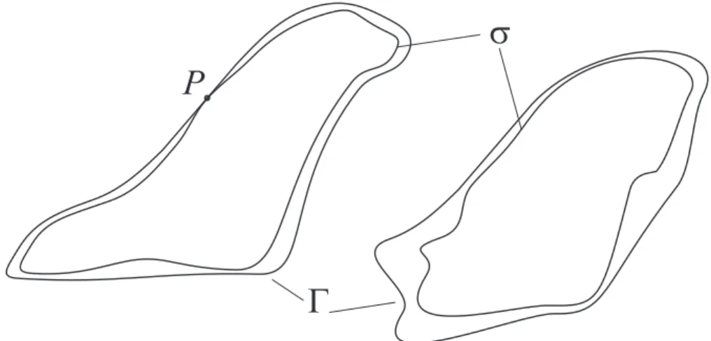
Letσ ={z∈C:|T_N(z)|= 1} be the level line of a polynomial T_N, and assume thatσ has no self-intersections. Let deg(T_N) =N.

The normal derivative of the Green’s function with pole at infinity of the outer domain to σ at a point z ∈ σ is (see [22, (2.2)]) |T_N^′ (z)|/N, and since this normal derivative is 2π-times the equilibrium density of σ (see [14, II.(4.1)] or [17, Theorem IV.2.3] and [17, (I.4.8)]), it follows that the equilibrium density onσ has the form

ω_σ(z) = |T_N^′ (z)|

2πN . (4.1)

Ifz∈σ, then there arenpointsz1, . . . , zn∈σwith the propertyTN(z) = T_n(z_k), and for them (see [22, (2.12)])

Z

σ

X^N

i=1

f(z_i)

|T_N^′ (z)|ds_σ(z) =N Z

σ

f(z)|T_N^′ (z)|ds_σ(z). (4.2) Furthermore, ifg:T→Cis arbitrary, then (see [22, (2.14)])

Z

σ

g(T_N(z))|T_N^′ (z)|ds_σ(z) =N Z 2π

0

g(e^it)dt. (4.3) Letz₀ ∈σ be arbitrary, and define the measure

dµ_σ(z) =|z−z₀|^αds_σ(z), α >−1, (4.4)

(19)

wheres_σ denotes the arc measure onσ. Without loss of generality we may assume thatT_N(z0) =e^iπ/2. Our plan is to compare the Christoffel functions for the measureµ_σ with that for the measureµ_α which is supported on the unit circle and is defined via

dµ_α(eît) =|eît−eîπ/2|^αdsT(eît), (4.5) and for which the asymptotics of the Christoffel function was calculated in (3.15).

We shall prove that

n→∞lim n^α+1λ_n(µ_σ, z₀) = L_α

(πω_σ(z₀))^α+1 (4.6) whereL_α is taken from (3.4).

4.1 The upper estimate

Let η > 0 be an arbitrary small number, and select a δ > 0 such that for everyz with|z−z₀|< δ, we have

1

1 +η|T_N^′ (z₀)| ≤ |T_N^′ (z)| ≤(1 +η)|T_N^′ (z₀)| 1

1 +η|T_N^′ (z₀)||z−z₀| ≤ |T_N(z)−T_N(z₀)| ≤(1 +η)|T_N^′ (z₀)||z−z₀| (4.7)

(note that T_N^′ (z₀) 6= 0 because σ has no self-intersections). Let Q_n be the extremal polynomial forλ_n(µ_α, e^iπ/2), whereµ_α is from (4.5). DefineR_n as

R_n(z) =Q_n(T_N(z))S_n,z₀_,L(z),

where S_n,z₀_,L is the fast decreasing polynomial given by Corollary 2.2 for the lemniscate setLenclosed byσ (and for any fixed 0< τ <1 in Corollary 2.2). Note that R_n is a polynomial of degree nN +o(n) with R_n(z₀) = 1.

SinceS_n,z₀_,L is fast decreasing, we have sup

z∈L\{t:|t−z0|<δ}|Sn,z0,L(z)|=O(qⁿ^τ⁰)

for some q < 1 and τ₀ > 0. The Nikolskii-type inequality in Lemma 2.7 when applied to two subarcs ofTwhich contain the upper resp. lower part of the unit circle, yields

kQ_nk^T ≤Cn^(1+|α|)/2kQ_nkL²(µα) ≤Cn^(1+|α|)/2. Therefore,

sup

z∈L\{t:|t−z0|<δ}|R_n(z)|=O(qⁿ^τ⁰^/2).

(20)

It follows that Z

|z−z0|≥δ|Rn(z)|²|z−z0|^αdsσ(z) =O(qⁿ^τ⁰^/2). (4.8) Using (4.7), we have

Z

|z−z0|<δ|R_n(z)|²|z−z₀|^αds_σ(z)

≤ Z

|z−z0|<δ|Q_n(T_N(z))|²|z−z₀|^αds_σ(z)

≤ (1 +η)^|α|+1

|T_N^′ (z₀)|^α+1 Z

|z−z0|<δ|Q_n(T_N(z))|²|T_N(z)−T_N(z₀)|^α|T_N^′ (z)|ds_σ(z)

≤ (1 +η)^|α|+1

|T_N^′ (z₀)|^α+1 Z 2π

0 |Q_n(eît)|²|eît−eîπ/2|^αdt

= (1 +η)^|α|+1λ_n(µ_α, e^iπ/2)

|T_N^′ (z₀)|^α+1 . This and (4.8) imply

λ_deg(R_n₎(µ_σ, z₀)≤(1 +η)^|α|+1 λ_n(µ_α, e^iπ/2)

|T_N^′ (e^iπ/2)|^α+1 +O(qⁿ^τ⁰^/2), from which

lim sup

n→∞ deg(Rn)^α+1λ_deg(R_n₎(µσ, z0)

≤lim sup

n→∞ (nN+o(n))^α+1(1 +η)^|α|+1λ_n(µ_α, e^iπ/2)

|T_N^′ (z₀)|^α+1

= (1 +η)^|α|+1 N^α+1

|T_N^′ (z₀)|^α+12^α+1L_α,

where we used (3.15). Since η > 0 is arbitrary, we obtain from (4.1) (use also (2.2))

lim sup

n→∞ n^α+1λ_n(µ_σ, z₀)≤ N^α+1

|T_N^′ (z₀)|^α+12^α+1L_α= L_α

(πω_σ(z₀))^α+1. (4.9) 4.2 The lower estimate

Let P_n be the extremal polynomial for λ_n(µ_σ, z₀), and let S_n,z₀_,L be the fast decreasing polynomial given by Corollary 2.2 for the closed lemniscate domainLenclosed by σ(with some fixedτ <1). As before, we obtain from Lemma 2.7

kP_nkσ =O(n^(1+|α|)/2). (4.10)

(21)

Define R_n(z) =P_n(z)S_n,z₀_,L(z). R_n is a polynomial of degreen+o(n) and Rn(z0) = 1. Similarly to the previous section, we have

sup

z∈L\{t:|t−z0|<δ}|Rn(z)|=O(qⁿ^τ⁰^/2) (4.11) for some q < 1 and τ₀ > 0. Since the expression PN

k=1R_n(z_k), where {z₁, . . . , z_N}=T_N⁻¹(T_N(z)), is symmetric in the variables z_k, it is a sum of their elementary symmetric polynomials. For more details on this idea, see [23]. Therefore, there is a polynomial Q_n of degree at most deg(R_n)/N = (n+o(n))/N such that

Qn(T_N(z)) = XN

k=1

Rn(z_k), z∈σ.

We claim that for every z∈σ, we have

|Q_n(T_N(z))|²≤ XN

k=1

|R_n(z_k)|²+O(qⁿ^τ⁰^/2). (4.12) Indeed, sinceσ has no self intersection, |zk−zl|cannot be arbitrarily small for distinct k and l. As a consequence, for every z at most one z_j belongs to the set{z : |z−z₀|< δ} ifδ is sufficiently small, and hence, in the sum

|Qn(TN(z))|² ≤ XN

k=1

XN

l=1

|Rn(z_k)||Rn(z_l)|, every term withk6=l isO(qⁿ^τ⁰^/2) (use (4.10) and (4.11)).

Now letδ >0 be so small that for everyzwith|z−z0|< δthe inequalities in (4.7) hold. Then (4.2) and (4.12) give (note thatT_N(z) =T_N(z_k) for all k)

Z

σ|Q_n(T_N(z))|²|T_N^′ (z)||T_N(z)−T_N(z₀)|^αds_σ(z)

≤O(qⁿ^τ⁰^/2) + Z

σ

XN

k=1

|R_n(z_k)|²

!

|T_N^′ (z)||T_N(z)−T_N(z₀)|^αds_σ(z)

=O(qⁿ^τ⁰^/2) + Z

σ

XN

k=1

|R_n(z_k)|²|T_N(z_k)−T_N(z₀)|^α

!

|T_N^′ (z)|ds_σ(z)

=O(qⁿ^τ⁰^/2) +N Z

σ|Rn(z)|²|T_N(z)−T_N(z0)|^α|T_N^′ (z)|dsσ(z)

≤O(qⁿ^τ⁰^/2) + (1 +η)^|α|+1|T_N^′ (z₀)|^α+1N Z

|z−z0|<δ|P_n(z)|²|z−z₀|^αds_σ

≤O(qⁿ^τ⁰^/2) + (1 +η)^|α|+1|T_N^′ (z₀)|^α+1N λ_n(µ_σ, z₀).

Christoﬀel functions with power type weights

Christoffel functions with power type weights

Contents

1 Introduction

G

G

2 Tools

3 The model cases

4 Lemniscates