Investigation of the liquid-vapour interface of aqueous methylamine solutions by computer simulation methods
Réka A. Horváth
a, Balázs Fábián
b,c,‡, Milán Szőri
d, Pál Jedlovszky
e,*
a
Apáczai Csere János School of the ELTE University, Papnövelde u. 4. H-1053 Budapest, Hungary
b
Department of Inorganic and Analytical Chemistry, Budapest University of Technology and Economics, Szt. Gellért tér 4, H-1111 Budapest, Hungary a
b
Institut UTINAM (CNRS UMR 6213), Université Bourgogne Franche-Comté, 16 route de Gray, F-25030 Besançon, France
d
Institute of Chemistry, University of Miskolc, Egyetemváros A/2, H-3515 Miskolc, Hungary
e
Department of Chemistry, Eszterházy Károly University, Leányka u. 6, H-3300 Eger, Hungary
Running title: Liquid-vapour interface of aqueous methylamine solutions
‡Present address: Institute of Organic Chemistry and Biochemistry of the Czech Academy of Sciences, Flemingovo nám. 2, CZ-16610 Prague 6, Czech Republic
*E-mail: jedlovszky.pal@uni-eszterhazy.hu
This document is the Accepted Manuscript version of a Published Work that appeared in final form in Journal of Molecular Liquids, copyright C Elsevier after peer review and technical editing by the publisher. To access the final edited and published work see:
https://www.sciencedirect.com/science/article/abs/pii/S0167732219318161
Abstract:
Molecular dynamics simulations of the liquid-vapour interface of water-methylamine mixtures of eight different compositions, including neat water, are performed on the canonical (N,V,T) ensemble at 280 K. The molecules constituting the first three individual molecular layers beneath the liquid surface are identified by the Identification of the Truly Interfacial Molecules (ITIM) method. The results indicate that methylamine molecules are strongly adsorbed in the first, and somewhat depleted in the second molecular layer, while the composition of the third layer agrees well with that of the bulk liquid phase. On the other hand, methylamine molecules do not show considerable self-association within the surface layer. The orientational preferences of the methylamine molecules at the liquid surface are clearly governed by the requirement of maximizing their hydrogen bonding interaction. As a consequence, methylamine molecules point by their apolar CH3 group straight to the vapour, while by the potential hydrogen bonding directions of the NH2 group flatly to the liquid phase. Further, within the surface layer, methylamine molecules stay, on average, noticeably farther from the bulk liquid phase than waters. Increasing methylamine mole fraction leads to the gradual breaking up of the lateral percolating H-bonding network of the surface molecules. Finally, methylamine molecules accelerate, while water molecules slow down the exchange of both species between the liquid surface and the bulk liquid phase. Further, methylamine molecules slow down the lateral diffusion of each other, and even prevent water molecules from showing noticeable lateral diffusion within the surface layer. The reason for this latter effect is that the mean residence time of the water molecules at the liquid surface becomes considerably shorter than the characteristic time of their lateral diffusion in the presence of methylamine.
Keywords: methylamine-water mixtures; intrinsic surface analysis; computer simulation;
liquid-vapour interface
1. Introduction
Among the roughly 150 amines that have already been identified in the atmosphere, the most common and abundant one is methylamine (CH3NH2) [1]. Amines are emitted from a wide range of natural as well as industrial sources, including biomass burning, protein degradation, vegetation, soils, ocean organisms, meat cooking, fish processing, motor vehicles, sewage treatment and waste incineration [2], as well as from recently introduced carbon capture and storage (CCS) devices [3,4]. Atmospheric formation of methylamine through oxidation and hydrolysis of trimethylamine has also been reported [5]. The global emission flux and total flux of methylamine is estimated to be 83 ± 26 Gg N yr−1 and 285 ± 78 Gg N yr−1, respectively [6]. Atmospheric concentration of amines can exceed several ppbv near their sources [1,6], but their background concentration is typically at the pptv to tens of pptv level in the gas phase [7] due to their fast oxidation by OH radicals and uptake by atmospheric particles [8]. Based on the reaction of methylamine with the OH radical, which is two order of magnitude faster than that of ammonia, the atmospheric lifetime of methylamine is estimated to be 25 hours [9], while this value is reduced to 5-10 hours taking also their uptake into account [2] (the steady-state uptake coefficient (γss) of methylamine is 6.0×10⁻³ at 293 K [10]).
Wet deposition is an important process to bring atmospheric methylamine to the surface of Earth [11] due to its high water solubility and strong basicity (pKb = 3.37 [9]).
Thus, methylamine can efficiently enter into condensed phases both via direct dissolution and acid–base reactions with organic [12] and inorganic acids [4]. Reaction of H2SO4 with amines represents the initial step in their gas-to-particle conversion, as it leads to the formation of small clusters [13] that can then further grow into detectable size particles in the atmosphere [14]. Amines can also react with atmospheric HNO3 to form particulate nitrate [15]. Despite their much lower ambient concentrations, among the few atmospheric bases, amines are thought to be comparable to ammonia in their contribution to new particle formation and growth, in part because they form stronger bonds with acids as compared with NH3, and also because they can efficiently replace the ammonium ion in particles taken up from the gas phase [14,16]. Therefore, detailed investigation of the adsorption of small amines at aqueous surfaces is an important part of the understanding of their gas-to-particle conversion.
Computer simulation studies can efficiently complement experimental investigations in addressing, among others, problems related to the structural and energetic properties of the bulk liquid phase as well as liquid-gas interface, since computer simulation methods can provide a full, atomistic level insight into the suitably chosen model of the system to be studied, while the model can only be validated against real experimental data [17]. Properties of liquid methylamine have also been studied by computer simulation methods several times in the bulk liquid phase. Thus, Kusalik et al. investigated the local structure around the methylamine molecules both in its neat liquid phase and aqueous solutions [18]. Kosztolányi et al. also investigated the local structure, including hydrogen bonding, in neat liquid methylamine using radial distribution functions and density projections of the neighbouring molecules. Comparison of the calculated radial distribution functions showed good agreement with results of neutron scattering experiments in the range of intermolecular distances [19].
Recently, Biswas and Mallik studied the bulk phase orientational preferences of the methylamine molecules in neat methylamine [20] as well as in its aqueous solution [21] at ambient conditions by first principles molecular dynamics simulations using dispersion corrected density functional (BLYP-D). Computer simulation studies of the behaviour of methylamine at aqueous interfaces are, however, rather scarce. Recently we studied the adsorption of methylamine at the surface of both crystalline [22] and amorphous [23] ice from the vapour phase. In these studies we demonstrated the strong tendency of methylamine molecules for being adsorbed at icy surfaces, including their ability even for multilayer adsorption, and characterized the surface orientation of the adsorbed molecules as well as their hydrogen bonding with the surface waters [22,23]. Hoehn et al. investigated the energetic and structural properties of a single methylamine molecule at air/water interface [24]. In this study, the solvation free energy profile of the methylamine molecule was found to exhibit a minimum at the interfacial region, whereas the magnitude of this effect (2.5-5.2 kJ/mol) was found to be rather sensitive to the force field combination used. Further, the interfacial orientation of methylamine as well as the hydrogen bonding characteristics of the water molecules surrounding the methylamine molecule at the interface of the infinitely dilute solution were also discussed [24]. However, we are not aware of any computer simulation study of the liquid-vapour interface of aqueous methylamine solutions of finite concentration, thus, to the best of our knowledge, the concentration effect on the interfacial properties of methylamine has been never discussed in the literature.
Meaningful computer simulation investigation of fluid (e.g., liquid-vapour and liquid- liquid) interfaces has long been hindered by the fact that the liquid surface is corrugated, on the molecular length scale, by the occurrence of capillary waves. [25] As a consequence, determining the list of the molecules that are located at the surface of their phase (i.e., being in contact also with the opposite phase), or, equivalently, finding the geometric covering surface, also called as the intrinsic surface, of the phase of interest is far from being a trivial task. Certainly, the simple association of the interfacial region with a macroscopically flat slab characterized by intermediate densities of the components between the two bulk phases was repeatedly shown to lead to a systematic error of unknown magnitude in the calculated interfacial properties (e.g., composition, orientation, dynamics, etc.) [26-29], and this systematic error can even propagate into the calculated thermodynamic properties of the system of interest [30]. The determination of the real, capillary wave corrugated intrinsic interface is further complicated by the fact that if the phase of interest consists of discrete particles (as it is the case in computer simulations), the intrinsic interface itself inherently depends on a free parameter that defines the length scale on which the interface is looked at [31].
The importance of the determination of the intrinsic liquid surface was already realized in the first simulations of liquid-liquid [32] and liquid-vapour [33] interfaces. In the early simulations, the intrinsic surface was estimated by dividing the basic box into several slabs perpendicular to the macroscopic plane of the interface, and determined the position of the liquid surface in each slab separately [32-35]. This method was later elaborated by Jorge and Cordeiro by determining the number of slabs required for convergence [36].
Alternatively, in cases when the list of the interfacial particles was already known (such as in simulations of lipid bilayers), the Voronoi cells of the projections of the interfacial atoms to the macroscopic plane of the interface were lifted back to the vertical positions of their central atoms [37]. The first systematic method of determining the intrinsic liquid surface was proposed by Chacón and Tarazona [38]. In this method, the intrinsic surface is defined as the covering surface of minimum area that goes through a set of pivot atoms, determined using a self-consistent procedure [38]. Following this pioneering work, several other methods have been proposed [26,31,36,39-43], some of which are even free from the assumption that the interface is macroscopically flat [39,41-43]. Among the various methods, the Identification of the Truly Interfacial Molecules (ITIM) [26] was shown to represent an excellent compromise between computational cost and accuracy [31]. Intrinsic surface analyzing methods have been
successfully applied in the past 15 years to the liquid-liquid and liquid-vapour interfaces of several neat molecular liquids [26,28-31,36,40,44-48] and their binary mixtures [27,49-55] as well as for aqueous electrolyte solutions [56], ionic liquids [57-61], mixtures of ionic and molecular liquids [62], aqueous surfaces covered by amphiphilic polymers [63,64] or surfactants [64-66] as well as for lipid membranes [67]. Further, profiles of several physical quantities, such as the density [36,38,45,68-71], energy [71], solvation free energy [72,73], electrostatic potential [56], and lateral pressure (or surface tension) [71,74] relative to the intrinsic liquid surface have been calculated in such systems.
In this paper, we present a detailed investigation of the properties of the intrinsic liquid surface of aqueous methylamine solutions of different compositions by means of molecular dynamics computer simulation and ITIM analysis. Properties of the interfacial layer as well as of the subsequent subsurface layers (e.g., width, separation, composition) as well as of the interfacial molecules (adsorption, orientation, hydrogen bonding, lateral diffusion and lateral self-association) are analyzed in detail. The paper is organized as follows. In section 2 details of the calculations performed, including the molecular dynamics simulations and ITIM analyses are given. The obtained results are discussed in detail in section 3. Finally, in section 4 the main conclusions of this study are summarized.
2. Computational details
2.1. Molecular dynamics simulations
Molecular dynamics simulations of the liquid-vapour interface of water-methylamine mixtures of different compositions have been performed on the canonical (N,V,T) ensemble at 280 K. The systems consisted of 4000 molecules, among which 0, 40, 120, 200, 400, 600, 800, and 1200 have been methylamine, thus, these systems correspond to the overall methylamine mole fraction, xMA, of 0, 0,01, 0.03, 0.05, 0.10, 0.15, 0.20, and 0.30, respectively. The X edge of the basic simulation box, being perpendicular to the macroscopic plane of the interface, has been 150 Å long, while the length of the Y and Z edges has been 50 Å in every case.
Methylamine molecules have been described by the generalized AMBER force field (GAFF) [75], using the fractional charges developed by Hoehn et al. [24], while water was
modelled by the TIP4P/2005 potential [76]. Besides describing the properties of the corresponding neat liquids well, this model combination was shown to reproduce the experimental hydration free energy of methylamine [77] within error bars [24]. Both potential models are rigid and pairwise additive, thus, the total energy of the system (apart from the long range correction) is given by the sum of the interaction energies of all molecule pairs.
The interaction energy of a molecule pair is simply the sum of the Lennard-Jones and charge- charge Coulomb contributions of all pairs of their atoms, given that the centres of the two molecules are closer to each other than a given cut-off distance, and it is zero otherwise. For this centre-centre cut-off distance we have chosen the value of 12.5 Å. The Lennard-Jones distance and energy parameters ( and , respectively), and fractional charges carried by the individual atoms, q, corresponding to the potential models used are summarised in Table 1.
Besides the O and H atoms, the TIP4P/2005 water model also consists of a virtual atom, denoted as M, as an additional interaction site. This virtual atom is located along the bisector of the H-O-H bond angle (being 104.52o) at 0.1546 Å from the O atom, while the O-H bond lengths are 0.9572 Å [76]. In the methylamine model used, the C-H, C-N, and N-H bonds are 1.10 Å, 1.47 Å, and 1.02 Å long, respectively, while the H-C-H, H-C-N, C-N-H, and H-N-H bond angles are 107.7o, 109.3o, 108.7o, and 105.0o, respectively [75].
The simulations have been performed using the GROMACS 5.1.4 program package [78]. Equations of motion have been integrated in time steps of 1 fs. The temperature of the systems has been controlled using the Nosé-Hoover thermostat [79,80]. The geometry of the molecules has been kept unchanged by the LINCS algorithm [81]. The long range part of the electrostatic interaction has been accounted for by the smooth particle mesh Ewald (sPME) method [82]. All systems have been equilibrated for 10 ns, followed by a 4 ns long production stage, in which 4000 sample configurations, separated from each other by 1 ps long trajectories, have been saved for the majority of the analyses. Further, another 1000 sample configurations per system, separated from each other by 0.1 ps long trajectories, have also been saved from a subsequent, 100 ps long production run for the analyses of the H-bond dynamics. Finally, all quantities calculated have been averaged not only over the sample configurations, but also over the two liquid-vapour interfaces present in the basic box.
2.2. ITIM analyses
In an ITIM analysis [26], the interfacial molecules are searched for by moving a spherical probe of a given radius along a set of test lines parallel with the macroscopic surface normal from the bulk opposite phase towards the surface to be determined. Once the probe hits the first particle that belongs to the phase of interest, this particle is marked as being at the interface (as it is “seen” by the probe from the opposite phase), and the next test line is considered. Once the procedure goes over all the test lines, the full list of the interfacial molecules is determined. Disregarding the determined full set of molecules and repeating the entire procedure allows also the determination of the molecules that form the subsequent molecular layer beneath the liquid surface.
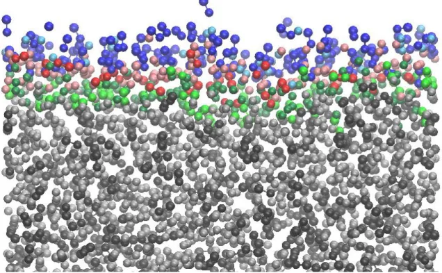
The ITIM analyses have been performed using the freely available [83] PYTIM package [84]. According to the suggestions of previous studies [26,31,85], here we have used a 125 × 125 grid of test lines, thus, neighbouring test lines have been separated from each other by 0.4 Å, and the radius of the probe sphere has been set to 2.0 Å. In determining whether an atom is touched by the probe sphere, the diameter of the atoms has been estimated by their Lennard-Jones distance parameter, . The ITIM procedure has been repeated three times, thus, the molecules forming the first three layers beneath the liquid surface have been determined. An equilibrium snapshot of the surface portion of the xMA = 0.30 system is shown in Figure 1, in which the molecules that belong to the first three molecular layers are also indicated.
3. Results and discussion
3.1. Surface tension
To further validate the potential model combination used, we have calculated the surface tension, , of the systems simulated. In order to avoid the error coming from the neglect of its ideal gas contribution, [86] surface tension has been calculated through the elements of the pressure tensor rather than those of the virial tensor, as [25]
=
X(
−)
0
L
N ( ) d
2 1L
X X p
p , (1)
where pN and pL are the normal and lateral components of the pressure tensor, respectively, LX
length of the X edge of the basic box, X is the position along this edge (i.e., the surface normal axis), and the factor of 1/2 accounts for the two liquid-vapour interfaces present in the basic box. It should be noted that while the value of pL can change along the surface normal, pN
must be constant due to the requirement of the mechanical stability of the system.
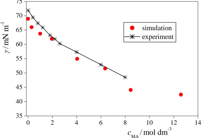
The obtained surface tension values are collected in Table 2, and are shown and compared with experimental values [87] in Figure 2. For this comparison, the bulk liquid phase methylamine concentration, cMA, has been calculated through the number of methylamine molecules in the 20 Å wide liquid slab in the middle of the bulk aqueous phase (i.e., at |X| < 10 Å). As is seen, the simulation results agree very well with the experimental data, their difference never exceeds 3 mN/m, and remains always below 5%.
3.2. Arrangement of the molecules
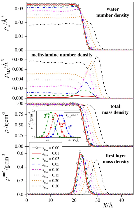
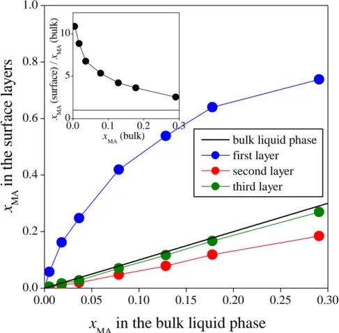
3.2.1. Arrangement along the interface normal. The number density profiles of the water and methylamine molecules as well as the mass density profiles of the entire system and the first molecular layer of the liquid phase along the macroscopic interface normal axis, X, are shown in Figure 3 as obtained in the eight different systems simulated. As is seen, the methylamine density profile exhibits a clear peak in the interfacial region, preceded by a minimum at the liquid side of the interface. Further, at least in the systems of high methylamine content, the water profiles exhibit a small but clear peak at the position of the minimum of the corresponding methylamine profile. These findings suggest that methylamine is adsorbed at the surface of its aqueous solution. To further analyze this point, and see how this adsorption affects the composition of the subsequent molecular layers beneath the liquid surface, we have calculated the methylamine mole fraction in the first three molecular layers as well as in the bulk liquid phase. This latter quantity has simply been obtained through the molecular number densities of the two components in the 20 Å wide liquid slab in the middle of the bulk aqueous phase. The methylamine mole fractions obtained in the first three molecular layers are shown as a function of the bulk phase methylamine mole fraction in Figure 4, and these values are also included in Table 2.
As is seen, the methylamine molecules are indeed accumulated in the surface molecular layer; this accumulation is stronger in more dilute systems, and progressively decreases with increasing bulk phase methylamine concentration (see Table 2 and the inset of Fig. 4). However, the surface adsorption of methylamine is strictly limited to the first layer, moreover, methylamine is even noticeably depleted in the second molecular layer, while the composition of the third subsurface layer is already essentially identical with that of the bulk liquid phase. In this respect, methylamine behaves in a markedly different way (i) than acetonitrile [49], HCN [52], and acetone [53], the adsorption of which involves several molecular layers beneath the surface of their aqueous solutions, (ii) than formamide, which is not adsorbed strongly at the surface of its aqueous solution [55], and (iii) also than methanol [27] and DMSO, [50] which are also strongly adsorbed in the first molecular layer, but do not show noticeable depletion in the second layer.
The comparison of the mass density profiles of the entire systems with those of the first molecular layer of the liquid phase reveals that the first layer extends well into the X range where the density of the entire system is already constant. Further, the density peak of the second and even the third layers extend to the X range characterized by intermediate densities between the bulk liquid and vapour phases. This finding clearly demonstrates the extent of the systematic error accompanying the identification of the liquid surface through the X range of intermediate densities, and stresses again the importance of performing intrinsic analysis of the liquid surface instead in such studies.
The density profiles of the individual layers can be very well fitted by Gaussian functions, in accordance with the theoretical claim of Chowdhary and Ladanyi [88] (see the inset of Fig. 3). The parameters corresponding to the peak position and width of these fitted Gaussians, X0 and G, respectively, can serve as an estimate of the average position and width of the corresponding molecular layers. The X0 and G parameters corresponding to the first three molecular layers of the eight systems simulated are also collected in Table 2. As is seen, the distance between the first two layers agrees very well with that of the second and third layer, the difference between these values remains below 3% in every case. However, although the subsequent molecular layers are equally spaced, the subsequent layers become more compact upon going towards the liquid phase, and this shrinking effect is particularly strong between the first two layers of the mixed systems. Thus, while in neat water the width of the subsequent molecular layers always decreases by about 5% upon going farther from the interface, in the mixed system this decrease is 7-10% between the first two, and only 1-5%
between the second and third layers. Moreover, the former value increases, while the latter decreases with increasing methylamine content. Considering the fact that all the three layers get thicker with increasing overall methylamine content, and also the above discussed adsorption of methylamine in the first, and depletion in the second molecular layer, these changes in the thickness of the subsequent subsurface layers can largely be accounted for by the larger size of the methylamine molecule than that of water.
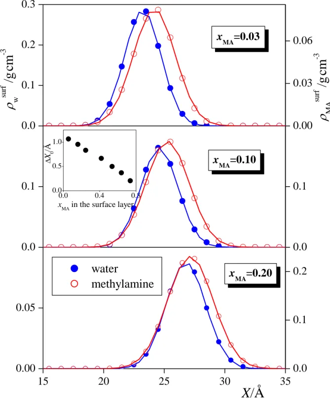
Figure 5 shows separately the mass density profiles of the water and methylamine molecules within the surface layer in the xMA = 0.03, 0.10, and 0.20 systems, together with their Gaussian fits. As is seen, the peak of the methylamine profile is located clearly, by about 0.5-1 Å closer to the vapour phase than that of the water molecules. This finding indicates that, within the surface layer, methylamine prefers to stay at the crests, while water is enriched in the troughs of the molecularly rough liquid surface. The distance between the peak positions of the Gaussian functions fitted to the profiles of the two components, X0, is shown as a function of the methylamine mole fraction in the first layer in the inset of Fig. 5.
As is seen, this outward shift of the methylamine peak with respect to that of water decreases linearly with the methylamine content of the first layer.
3.2.2. Arrangement within the surface layer. In this section, we address the question whether, besides their accumulation in the surface layer, the methylamine molecules also exhibit considerable lateral self-association within this layer. For this purpose, we have projected the centre of mass of the methylamine molecules belonging to the surface layer into the macroscopic plane of the surface, YZ, and calculated the area distribution of the Voronoi cells of these projections, A. For a set of planar seeds (in our case, the projections), the Voronoi cell of a given seed is the locus of points in the plane that are closer to this seed than to any other one [89-91]. If the seeds are homogeneously arranged in the plane, the distribution of the area of the Voronoi cells follows a gamma distribution [29,92,93]:
P(A)=aA−1exp(−A), (2)
which, if small areas occur with low enough probabilities, approaches a Gaussian distribution [94]. In this equation, and are free parameters, while a normalizes the distribution to unity. However, if the seeds are arranged in a correlated way, forming dense patches (i.e.,
self-associates) and leaving large empty areas, the P(A) distribution deviates from eq. 2, exhibiting a long, exponentially decaying tail at its high A side [94].
The P(A) distributions obtained in selected systems, together with their best fits obtained using eq. 2 are shown in Figure 6. As is seen, the obtained distributions can be very well fitted by eq. 2, with the exception of the system of the lowest methylamine content considered. In this latter case, the P(A) distribution deviates noticeably from its best fit, and exhibits an exponentially decaying tail (transformed to a straight line using the logarithmic scale for the distribution) at its large A side. However, in interpreting this result it has to be emphasized that in the surface layer of the xMA = 0.01 system only about 6% of the molecules are methylamine (see Table 2), and hence small associates of a few methylamine molecules, not necessarily being even contact positions, might already well account for this deviation.
This finding reveals that, similarly to DMSO [54] and formamide [55], but in contrast with acetonitrile [49] and HCN [52], the methylamine molecules do not show considerable self- association at the surface of their aqueous solution.
3.3. Surface orientation
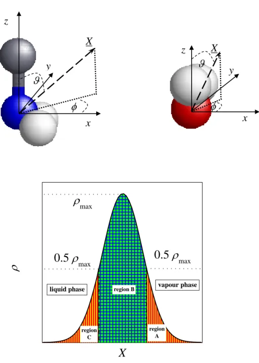
Since the relative orientation of a rigid body (e.g., a molecule) relative to an external direction (e.g., the macroscopic surface normal axis) can fully be described only by using two independent orientational variables, the full description of the orientational statistics of such molecules requires the calculation of the bivariate joint probability distribution of these two independent orientational variables [95,96]. We showed that the two angular polar coordinates of the surface normal vector in a local Cartesian frame fixed to the individual molecules is a sufficient choice of this independent orientational variable pair [95,96]. However, it has to be kept in mind that the polar angle is formed by two general spatial vectors (i.e., the z axis of the local frame and the macroscopic surface normal), but is the angle of two vectors (i.e., the x axis of the local frame and the projection of the macroscopic surface normal to the xy plane of this frame) that lay, by definition, in a given plane (i.e., the xy plane of the local frame). Therefore, uncorrelated orientation of the molecules with the surface results in a uniform bivariate distribution only if cos and are chosen to be the orientational variables.
In this study, we define the local Cartesian frames in the following way. In the case of methylamine, its origin is the N atom, axis z points from the N to the C atom along the N-C bond, axis y is parallel with the line joining the two H atoms of the NH2 group, while axis x is
perpendicular to both y and z, and it is oriented in such a way that the x coordinates of the NH2 hydrogen atoms are positive. For water, the origin of the local frame is the O atom, axis z is the symmetry axis of the molecule, oriented in such a way that the z coordinates of the H atoms are positive, x is the molecular normal axis, and axis y is perpendicular to both x and z.
Due to the symmetry of the methylamine and water molecules, these frames are always chosen according to the inequalities < 180o (for methylamine) and < 90o (for water). The definition of these local frames as well as that of the polar angles and of the surface normal vector, X (oriented, by our convention, by pointing towards the vapour phase) in these frames are illustrated in Figure 7.
In order to investigate also the influence of the local curvature of the surface on the orientational preferences of the surface molecules, the surface layer has been divided to three separate regions, and the bivariate distribution of the orientational variables cos and has been calculated not only in the entire surface layer, but also in its separate regions A, B, and C. These regions are defined in the following way. Region B covers the X range where the density of the first layer exceeds half of its maximum value, while regions A and C, corresponding typically to the crests (surface portions of positive local curvature) and troughs (those of negative local curvature) of the molecularly rough liquid surface, are located at the vapour and liquid side of region B, respectively. The definition of regions A, B, and C of the surface layer is also illustrated in Fig. 7.
The P(cos,) orientational maps of the surface methylamine and water molecules are shown in Figures 8 and 9, respectively, as obtained in the entire surface layer as well as in its separate regions A, B, and C of selected systems. The methylamine molecules prefer the orientation corresponding to the cos value of 1 in the entire surface layer as well as in its individual regions A, B, and C. In this alignment, marked here as IMA, the N-C bond stays perpendicular to the macroscopic plane of the surface in such a way that the NH2 group points straight to the liquid, while the CH3 group to the vapour phase. This orientation is illustrated in Figure 10. It should be noted that in the case of cos = 1 the macroscopic surface normal vector, X, points along the z axis of the local Cartesian frame, and hence its projection to the xy plane becomes a single point, and hence the polar angle loses its meaning (see Fig. 7).
This observed orientational preference is not at all surprising, since in this way the apolar CH3
groups of the methylamine molecules are exposed to the vapour phase, while the polar NH2
groups turn to the bulk liquid phase, and thus can still form up to three hydrogen bonds with
the neighbouring molecules, as both of their N-H bonds as well as the lone pair direction points flatly towards the bulk liquid phase.
In neat water, the molecules prefer the orientation corresponding to the cos = 0,
= 0o point of the P(cos,) orientational map in the entire surface layer as well as in its highest populated region, B. This orientation is marked here as Iw. However, in regions A and C, i.e., at the positively curved crests and negatively curved troughs, respectively, of the molecularly rough liquid surface, the peak corresponding to this preferred orientation is shifted somewhat to negative and positive cos values, respectively. This shift corresponds to a small flip of the two H atoms towards the bulk liquid phase (in region A), and towards the vapour phase (in region C). The corresponding orientations are denoted here as IAw and ICw, respectively. Further, in region A the orientation corresponding to cos = 0.3 and = 90o (marked here as IIw), while in region C that corresponding to cos = -0.3 and = 90o (marked here as IIIw) are also preferred. These preferred water alignments are also illustrated in Fig. 10. As it has been discussed previously [26-28], these orientational preferences of the surface molecules are guided by the requirement of these molecules maximizing their hydrogen bonds. Thus, at the positively curved crests (region A), three H-bonds of a water molecule can safely be maintained by sacrificing the fourth one. This is done by pointing either on of the two potential H-acceptor directions (in alignment IAw) or one of the two OH bonds (in alignment IIw) straight to the vapour phase, while the other three H-bonding directions point flatly toward the bulk liquid phase. On the other hand, at the troughs in region C, water molecules can maintain all their four possible H-bonds by straddling three hydrogen bonding directions (i.e., two OH bonds and a H-acceptor lone pair direction in alignment ICw, or one OH bond and both H-acceptor lone pair directions in alignment IIIw) flatly by the negatively curved portion of the surface, while the fourth possible H-bonding direction points straight to the liquid phase. As is seen this pattern of the surface orientational preferences of water more or less prevails with increasing methylamine content, although the peak corresponding to orientation IIw vanishes, while that corresponding to alignment IIIw broadens gradually.
It should be noticed that a methylamine molecule, aligned in its preferred surface orientation, can easily form hydrogen bonds with its water neighbours. Indeed, while in this alignment, methylamine points with both of its N-H bonds and with its lone pair direction flatly toward the bulk liquid phase, water molecules in orientations ICw and IIIw point three out of their four possible H-bonding directions flatly towards the vapour phase. The arrangements of these possible H-bonding methylamine-water pairs in the surface layer are also illustrated in Fig. 10. Since the methylamine molecules have two H-donating N-H groups pointing to the liquid, while water molecules in alignment IIIw have two H-accepting directions pointing to the vapour phase, H-bonded pairs formed by a methylamine molecule of alignment IMA and a water molecule of alignment IIIw are expected to be highly populated. This is in a clear accordance with the observed broadening of the IIIw peak of the water orientational map with increasing methylamine concentration. Further, the previous observation that, within the surface layer, methylamine molecules stay, on average, farther from the bulk liquid phase than waters (see Fig. 5), is also in a clear accordance with this picture.
3.4. Hydrogen bonding at the liquid surface
To further analyze hydrogen bonding between the molecules at the liquid surface, we have calculated the size distribution of the hydrogen bonding clusters of the molecules within the surface layer of the eight systems simulated. In this analysis, two molecules (irrespective of whether they are water or methylamine) are regarded as being hydrogen bonded to each other if the distance of their H-bonding heavy (i.e., oxygen or nitrogen) atoms is less than 3.4 Å, and that of the bonding H from its acceptor (i.e., O or N) heavy atom is less than 2.5 Å.
These threshold values correspond to the first minimum position of the corresponding radial distribution functions. Two molecules belong to the same cluster if they are connected through a chain of mutually H-bonding molecule pairs within the surface layer. It should be emphasized that two molecules that are not belonging to the same cluster according to this definition might still well be connected by a chain of H-bonding molecules, which contains also molecules that are located beneath the first molecular layer. However, here we are interested only in the hydrogen bonding clusters of the surface molecular layer. Finally, the size of a cluster is simply given by the number of molecules it consists, n.
At the percolation threshold, the distribution of the size of the existing clusters, P(n), follows a power law decay, i.e.,
P(n)~n−, (3)
where the universal exponent, , is 2.05 in two-dimensional systems [97]. In percolating systems, the P(n) distribution exceeds this critical value at large cluster sizes, while in systems that are below the percolation threshold P(n) drops below the critical line already at very small n values, and remains below it in the entire n range [98].
The P(n) distribution obtained in the systems of eight different compositions simulated are shown in Figure 11, together with the critical line of eq. 3. As it has been discussed several times [26-28,44,99-101], the molecules at the surface of neat liquid water clearly form a laterally percolating H-bonding network at this temperature. However, the addition of methylamine to the system leads to a gradual breakup of this lateral network: while the systems of overall methylamine mole fractions of 0.01 and 0.03 are still exhibit surface percolation, the xMA = 0.05 system (corresponding to the bulk liquid phase methylamine mole fraction of 0.037, see Table 2) is already around the percolation threshold, and in systems of higher methylamine content the liquid surface no longer contains a percolating H-bonding network of the molecules. In this respect, the aqueous solution of methylamine behaves similarly to that of DMSO [50], but differently from that of formamide, in which the molecules form a mixed percolating H-bonding lateral network at the liquid surface at any composition [55].
3.5. Dynamics of the molecules at the liquid surface
3.5.1. Mean surface residence time. To investigate also the dynamical properties of the surface molecules, we have calculated their mean residence time at the surface layer as well as their lateral diffusion coefficient within the surface molecular layer. The mean surface residence time of the molecules, surf, can be defined through the survival probability of the molecules in the surface layer, L(t), which is simply defined as the probability that a molecule that belongs to the surface layer at t0 will remain in this layer up to t0+t. Since the departure of the molecules from the surface layer is a process of first order kinetics, L(t) is expected to
follow an exponential decay. However, molecules can departure from the liquid surface by two different mechanisms. Thus, they can either leave the surface temporarily due to a fast oscillatory move and return to it quickly due to the same oscillation, or leave it permanently by diffusing to the bulk liquid phase. Therefore, we have fitted the simulated L(t) data by a biexponential function, i.e.,
) / exp(
) / exp(
)
(t A1 t osc A2 t surf
L = − + − , (4)
where osc is the time scale of the fast oscillatory move, and surf is the mean surface residence time of the molecules. The L(t) data obtained from the simulations together with their biexponential fits are shown in Figure 12 both for the water and methylamine molecules. As is seen, the simulated data can always be very well fitted by eq. 4. Further, osc has turned out to be indeed at least an order of magnitude smaller than surf in every case, in accordance with our above explanation.
The surf values obtained from the biexponential fit of the L(t) data are collected in Table 3. As is seen, methylamine molecules stay considerably (i.e., about an order of magnitude) longer at the liquid surface than water molecules in every composition. Further, the mean surface residence time of both molecules clearly decreases with increasing methylamine concentration. Thus, methylamine accelerates, while water slows down the exchange of both molecules between the surface layer and the bulk liquid phase of their mixtures.
3.5.2. Lateral diffusion of the surface molecules. The value of surf sets the time scale within which any molecular process can occur at the liquid surface. Thus, when studying the lateral diffusion of the molecules within the surface layer, first it has to be clarified whether the time scale of this diffusion is smaller or larger than surf. In the first case, surface molecules indeed exhibit considerable diffusion during their stay at the liquid surface.
However, if the time scale of the diffusion is larger than the mean surface residence time, molecules do not diffuse within the surface layer, simply because they leave the liquid surface before they could move considerably away from their starting position.
The lateral diffusion coefficient of the molecules, D||, can simply be evaluated using the Einstein relation [17], i.e.,
t D MSD
|| = 4 , (5)
where MSD is the mean square displacement of the molecules within the macroscopic plane of the liquid surface, YZ, and the factor 4 in the denominator reflects the fact that the diffusion is two-dimensional. The characteristic time of the surface diffusion, D, can be defined as the time during which the molecules explore a surface portion equal to the average surface area per molecule, Am. Thus, D can be calculated as [29,102]
= =
surf
||
Z Y
||
D m
2
4 D N
L L D
A , (6)
where LY and Lz are the Y and Z edge lengths of the basic box, respectively, while <Nsurf> is the mean number of the surface molecules in the basic box. It should be noted that eq. 6 accounts also for the two liquid surfaces present in the basic box.
To obtain the value of D||, the MSD(t) data resulted from the simulations have been fitted by a straight line. However, the first 5 ps (for water) and 10 ps (for methylamine) of these data have been left out from the fitting in order to ensure that the molecules have already left the ballistic regime and their mobility is governed by diffusive motion. The MSD(t) data along with their linear fit are shown in Figure 13 as obtained for both the water and the methylamine molecules in selected systems, while the obtained D|| values are included in Table 3. Due to the large difference in the molecular size, and hence also in the molecular surface area of water and methylamine, we have estimated Am of the water molecules by the value obtained in the xMA = 0.00 system (i.e., neat water) of 12.12 Å2. For methylamine, we have extrapolated the Am values, obtained without distinguishing the two molecules in the eight systems simulated, to xMA = 1.00. Thus, for methylamine, we have used the Am value of 21.24 Å2 in every system. The D values obtained this way are also included in Table 3.
As is seen, the D value of both molecules increases with increasing methylamine mole fraction. More importantly, while the relation D < surf holds for methylamine in all systems,
for water this relation is true only in neat water, in the xMA = 0.01 system the two time scales are roughly equal, and in systems of higher methylamine content D is clearly larger than surf. This finding means that in systems containing methylamine the water molecules do not show noticeable surface diffusion simply because they leave the surface layer earlier. On the other hand, methylamine molecules do exhibit considerable lateral diffusion at the liquid surface;
however, this diffusion becomes progressively slower with increasing methylamine content.
In other words, methylamine molecules slow down the diffusion of each other, and even immobilize the water molecules (i.e., prevent them from diffusion) within the surface layer of their aqueous solutions.
4. Summary and conclusions
In this paper, we have studied in detail the liquid-vapour interface of aqueous methylamine solutions of various concentrations at the molecular level by molecular dynamics simulations. The real, capillary wave corrugated intrinsic liquid surface as well as the subsequent molecular layers have been identified by the ITIM method [26]. The surface tensions of the simulated systems are in an excellent agreement with experimental data.
The results have revealed the strong affinity of the methylamine molecules to the liquid surface. On the other hand, methylamine molecules are noticeably depleted from the second layer, and the composition of only the third subsurface molecular layer agrees reasonably well with that of the bulk liquid phase. In this respect, the aqueous solution of methylamine behaves in a markedly different way from that of acetonitrile [49], HCN [52], and acetone [53], the adsorption of which involves several molecular layers, that of methanol [27] and DMSO [50], the adsorption of which involves also only the first molecular layer, however, no depletion of them occurs in the second layer, and also that of formamide [55], which shows no considerable adsorption even in the first molecular layer. However, in contrast with their clear preference for staying at the liquid surface, no considerable tendency of self-association of the methylamine molecules has been seen in the surface layer.
Besides being adsorbed in the surface molecular layer, methylamine molecules stay, on average, also noticeably (i.e., 0.5-1 Å) farther from the bulk liquid phase than water molecules even within the surface layer, and this effect has been found to be more marked in
more dilute solutions. This finding is explained by the requirement that surface molecules should maximize their hydrogen bonding. Thus, surface methylamine molecules strongly prefer the alignment in which the apolar CH3 group points straight to the vapour, while the possible H-bonding directions of the NH2 group flatly to the liquid phase. In this alignment, methylamine molecules can easily form hydrogen bonds with neighbouring waters that are located somewhat closer to the bulk liquid phase. It is also found that increasing methylamine concentration gradually breaks up the lateral percolating hydrogen bonding network of the surface molecules.
Analyzing the dynamics of the individual molecules we have found that methylamine accelerates, while water slows down the exchange of both molecules between the surface layer and the bulk liquid phase. Further, methylamine molecules slow down the lateral diffusion of each other, and even immobilize water molecules within the surface layer. As a consequence, during their rather short lifetime at the liquid surface, water molecules have no time to show noticeable lateral diffusion within the surface layer of these mixtures.
As it has been mentioned earlier, among the few atmospheric bases, amines are thought to be comparable to ammonia in their contribution to new particle formation and growth [14]. By using methylamine as an example for atmospheric organic amine, we can conclude that its enhanced surface propensity, measured by the ratio of the first layer and bulk phase methylamine mole fractions, is about five times higher than that of ammonia [103] at atmospherically more relevant low bulk concentrations (i.e., below 1%, as in the xMA = 0.01 system, see Table 2.). In addition, this effect can be even more pronounced for the more lipophilic (hydroapathic) larger amines (e.g. dimethylamine). Further, due to its preferred interfacial orientation, methylamine can easily interact with atmospheric acidic compounds approaching the liquid surface from the bulk liquid phase, making the amine ready to react (e.g. donating proton). These features may, in part, explain the enhanced particle formation ability of organic amines in the atmosphere.
Acknowledgements
The authors acknowledge financial support from the Hungarian NKFIH Foundation, under project number 119732. This research was supported by the European Union and the Hungarian State, co-financed by the European Regional Development Fund in the framework of the GINOP-2.3.4-15-2016-00004 project, aimed to promote the cooperation between the
higher education and the industry. M. Sz. gratefully acknowledges the financial support from the János Bolyai Research Scholarship of the Hungarian Academy of Sciences (BO/00113/15/7), and from the New National Excellence Program of the Ministry of Human Capacities (ÚNKP-17-4-III-ME/26). B. F. gratefully acknowledges the financial support from the New National Excellence Program of the Ministry of Human Capacities (ÚNKP-17-3-I).
References
[1] X. L. Ge, A. S. Wexler, S. L. Clegg, Atmos. Environ. 45 (2011) 524.
[2] F. Yu, G. Luo, Atmos. Chem. Phys. 14 (2014) 12455.
[3] C. J. Nielsen, H. Herrmann, C. Weller, Chem. Soc. Rev. 41(2012) 6684.
[4] S. M. Murphy, A. Sorooshian, J. H. Kroll, N. L. Ng, P. Chhabra, C. Tong, J. D.
Surratt, E. Knipping, R. C. Flagan, J. H. Seinfeld, Atmos. Chem. Phys. 7 (2007) 2313.
[5] M. L. Dawson, M. E. Varner, V. Perraud, M. J. Ezell, J. Wilson, A. Zelenyuk, R. B.
Gerber, B. J. Finlayson-Pitts, J. Phys. Chem. C 118 (2014) 29431.
[6] G. W. Schade, P. J. Crutzen, J. Atmos. Chem. 22 (1995) 319.
[7] Y. You, V. P. Kanawade, J. A. de Gouw, A. B. Guenther, S. Madronich, M. R. Sierra- Hernández, M. Lawler, J. N. Smith, S. Takahama, G. Ruggeri, A. Koss, K. Olson, K.
Baumann, R. J. Weber, A. Nenes, H. Guo, E. S. Edgerton, L. Porcelli, W. H. Brune, A. H.; Goldstein, S. H. Lee, Atmos. Chem. Phys. 14 (2014) 12181.
[8] S. A. Carl, J. N. Crowley, J. Phys. Chem. A 102 (1998) 8131.
[9] S. W. Gibb, R. Fauzi, C. Mantoura, P. S. Liss, Global Biogeochem. Cycles 13 (1999) 161.
[10] Q. Qiu, L. Wang, V. Lal, A. F. Khalizov, R. Zhang, Environ. Sci. Technol. 45 (2011) 4748.
[11] C. Qiu, R. Zhang, Phys. Chem. Chem. Phys. 15 (2013) 5738.
[12] K. C. Barsanti, J. F. Pankow, Atmos. Environ. 40 (2006) 6676.
[13] R. Zhang, A. Khalizov, L. Wang, M. Hu, W. Xu, Chem. Rev. 112 (2012) 1957.
[14] H. Chen, M. E. Varner, R. B. Gerber, B. J. Finlayson-Pitts, J. Phys. Chem. B 120 (2016) 1526.
[15] M. Kumar, H. Li, X. Zhang, X. C. Zeng, J. S. Francisco, J. Am. Chem. Soc. 140 (2018) 6456.
[16] X. L. Ge, A. S. Wexler, S. L. Clegg, Atmos. Environ. 45 (2011) 561.
[17] M. P. Allen, D. J. Tildesley, Computer Simulation of Liquids, Clarendon Press, Oxford, 1987.
[18] P. G. Kusalik, D. Bergman, A. Laaksonen, J. Chem. Phys. 113 (2000) 8036.
[19] T. Kosztolányi, I. Bakó, G. Pálinkás, J. Chem. Phys. 118 (2003) 4546.
[20] S. Biswas, B. S. Mallik, Phys. Chem. Chem. Phys. 19 (2017) 9912.
[21] S. Biswas, B. S. Mallik, ChemistrySelect 2 (2017) 74.
[22] V. Szentirmai, M. Szőri, S. Picaud, P. Jedlovszky, J. Phys. Chem. C 120 (2016) 23480.
[23] R. A. Horváth, Gy. Hantal, S. Picaud, M. Szőri, P. Jedlovszky, J. Phys. Chem. A 122 (2018) 3398.
[24] R. D. Hoehn, M. A. Carignano, S. Kais, C. Zhu, J. Zhong, X. C. Zeng, J. S. Francisco, I. Gladich, J. Chem. Phys. 144 (2016) 214701.
[25] J. S. Rowlinson, B. Widom, Molecular Theory of Capillarity, Dover Publications, Mineola, 2002.
[26] L. B. Pártay, G. Hantal, P. Jedlovszky, Á. Vincze, G. Horvai, J. Comp. Chem. 29 (2008) 945.
[27] L. B. Pártay, P. Jedlovszky, Á. Vincze, G. Horvai, J. Phys. Chem. B. 112 (2008) 5428.
[28] G. Hantal, M. Darvas, L. B. Pártay, G. Horvai, P. Jedlovszky, J. Phys.: Condens.
Matter 22 (2010) 284112.
[29] B. Fábián, M. Sega, G. Horvai, P. Jedlovszky, J. Phys. Chem. B. 121 (2017) 5582.
[30] L. B. Pártay, G. Horvai, P. Jedlovszky, J. Phys. Chem. C. 114 (2010) 21681.
[31] M. Jorge, P. Jedlovszky, M. N. D. S. Cordeiro, J. Phys. Chem. C 114 (2010) 11169.
[32] P. Linse, J. Chem. Phys. 86 (1987) 4177.
[33] I. Benjamin, J. Chem. Phys. 97 (1992) 1432.
[34] I. Benjamin, J. Chem. Phys. 110 (1999) 8070.
[35] D. Michael, I. Benjamin, J. Chem. Phys. 114 (2001) 2817.
[36] M. Jorge, M. N. D. S. Cordeiro, J. Phys. Chem. C 111 (2007) 17612.
[37] S. A. Pandit, D. Bostick, M. L. Berkowitz, J. Chem. Phys. 119 (2003) 2199.
[38] E. Chacón, P. Tarazona, Phys. Rev. Lett. 91 (2003) 166103.
[39] M. Mezei, J. Mol. Graphics Modell. 21 (2003) 463.
[40] J. Chowdhary, B. M. Ladanyi, J. Phys. Chem. B 110 (2006) 15442.
[41] A. P. Wilard, D. Chandler, J. Phys. Chem. B 114 (2010) 1954.
[42] M. Sega, S. S. Kantorovich, P. Jedlovszky M. Jorge, J. Chem. Phys., 138 (2013) 044110.
[43] J. Škvor, J. Škvára, J. Jirsák, I. Nezbeda J. Mol. Graphics Mod. 76 (2017) 17.
[44] L. B. Pártay, G. Horvai, P. Jedlovszky, Phys. Chem. Chem. Phys. 10 (2008) 4754.
[45] M. Jorge, M. N. D. S. Cordeiro, J. Phys. Chem. B 112 (2008) 2415.
[46] Gy. Hantal, P. Terleczky, G. Horvai, L. Nyulaszi, P. Jedlovszky, J. Phys. Chem. C 113 (2009) 19263.
[47] M. Darvas, K. Pojják, G. Horvai, P. Jedlovszky, J. Chem. Phys. 132 (2010) 134701.
[48] P. Jedlovszky, B. Jójárt, G. Horvai, Mol. Phys. 113 (2015) 985.
[49] L. B. Pártay, P. Jedlovszky, G. Horvai, J. Phys. Chem. C. 113 (2009) 18173.
[50] K. Pojják, M. Darvas, G. Horvai, P. Jedlovszky, J. Phys. Chem. C. 114 (2010) 12207.
[51] M. Darvas, L. B. Pártay, G. Horvai, P. Jedlovszky, J. Mol. Liquids 153 (2010) 88.
[52] B. Fábián, M. Szőri, P. Jedlovszky, J. Phys. Chem. C 118 (2014) 21469.
[53] B. Fábián, B. Jójárt, G. Horvai, P. Jedlovszky, J. Phys. Chem. C. 119 (2015) 12473.
[54] B. Fábián, A. Idrissi, B. Marekha, P. Jedlovszky, J. Phys.: Condens. Matter 28 (2016) 404002.
[55] B. Kiss, B. Fábián, A. Idrissi, M. Szőri, P. Jedlovszky, J. Phys. Chem. C. 122 (2018) 19639.
[56] F. Bresme, E. Chacón, P. Tarazona, A. Wynveen, J. Chem. Phys. 137 (2012) 114706.
[57] Gy. Hantal, M. N. D. S. Cordeiro, M. Jorge, Phys. Chem. Chem. Phys. 13 (2011) 21230.
[58] M. Lísal, Z. Posel, P. Izák, Phys. Chem. Chem. Phys. 14 (2012) 5164.
[59] Gy. Hantal, I. Voroshylova, M. N. D. S. Cordeiro, M. Jorge, Phys. Chem. Chem.
Phys. 14 (2012) 5200.
[60] M. Lísal, P. Izák, J. Chem. Phys. 139 (2013) 014704.
[61] Gy. Hantal, M. Sega, S. Kantorovich, C. Schröder, M. Jorge, J. Phys. Chem. C. 119 (2015) 28448.
[62] M. Sega, Gy. Hantal, Phys. Chem. Chem. Phys. 19 (2017) 18968.
[63] M. Darvas, T. Gilányi, P. Jedlovszky, J. Phys. Chem. B. 114 (2010) 10995.
[64] M. Darvas, T. Gilányi, P. Jedlovszky, J. Phys. Chem. B. 115 (2011) 933.
[65] N. Abrankó-Rideg, M. Darvas, G. Horvai, P. Jedlovszky, J. Phys. Chem. B 117 (2013) 8733.
[66] N. Abrankó-Rideg, G. Horvai, P. Jedlovszky, J. Mol. Liquids 205 (2015) 9.
[67] E. A. Shelepova, A. V. Kim, V. P. Voloshin, N. N. Medvedev, J. Phys. Chem. B 122 (2018) 9938.
[68] E. Chacón, P. Tarazona, J. Phys.: Condens. Matter 17 (2005) S3493.
[69] P. Tarazona, E. Chacón, Phys. Rev. B 70 (2004) 235407.
[70] M. Jorge, Gy. Hantal, P. Jedlovszky, M. N. D. S. Cordeiro, J. Phys. Chem. C. 114 (2010) 18656.
[71] M. Sega, B. Fábián, P. Jedlovszky, J. Chem. Phys. 143 (2015) 114709.
[72] M. Darvas, M. Jorge, M. N. D. S. Cordeiro, S. S. Kantorovich, M. Sega, P.
Jedlovszky, J. Phys. Chem. B 117 (2013) 16148.
[73] M. Darvas, M. Jorge, M. N. D. S. Cordeiro, P. Jedlovszky, J. Mol. Liquids 189 (2014) 39.
[74] M. Sega, B. Fábián, G. Horvai, P. Jedlovszky, J. Phys. Chem. C 120 (2016) 27468.
[75] J. Wang, R. M. Wolf, J. W. Caldwell, P. A. Kollman, D. A. Case, J. Comp. Chem. 25 (2004) 1157.
[76] J. L. F. Abascal, C. Vega, J. Chem. Phys. 123 (2005) 234505.
[77] R. Sander, Atmos. Chem. Phys. 15 (2015) 4399.
[78] S. Pronk, S. Páll, R. Schulz, P. Larsson, P. Bjelkmar, R. Apostolov, M. R. Shirts, J. C.
Smith, P. M. Kasson, D. van der Spoel, B. Hess, E. Lindahl, Bioinformatics 29 (2013) 845.
[79] S. Nosé, Mol. Phys. 52 (1984) 255.
[80] W. G. Hoover, Phys. Rev. A 31 (1985) 1695.
[81] B. Hess, J. Chem. Theory Comput. 4 (2008) 116.
[82] U. Essman, L. Perera, M. L. Berkowitz, T. Darden, H. Lee, L. G. Pedersen, J. Chem.
Phys. 103 (1995) 8577.
[83] URL: https://github.com/Marcello-Sega/pytim
[84] M. Sega, Gy. Hantal, B. Fábián, P. Jedlovszky, J. Comp. Chem. 39 (2018) 2118.
[85] M. Sega, Phys. Chem. Chem. Phys. 18 (2016) 23354.
[86] M. Sega, B. Fábián, P. Jedlovszky, J. Phys. Chem. Letters 8 (2017) 2608.
[87] B. T. Mmereki, J. M. Hicks, D. J. Donaldson, J. Phys. Chem. A 104 (2000) 10789.
[88] J. Chowdhary, B. M. Ladanyi, Phys. Rev. E 77 (2008) 031609.
[89] G. F. Voronoi, J. Reine Angew. Math. 134 (1908) 198.
[90] A. Okabe, B. Boots, K. Sugihara, S. N. Chiu, Spatial Tessellations: Concepts and Applications of Voronoi Diagrams, John Wiley, Chichester, 2000.
[91] N. N. Medvedev, The Voronoi-Delaunay Method in the Structural Investigation of Non-Crystalline Systems, SB RAS, Novosibirsk, 2000, in Russian.
[92] T. Kiang, Z. Astrophys. 63 (1966) 433.
[93] E. Pineda, P. Brunna, D. Crespo, Phys. Rev. E. 70 (2004) 066119.
[94] L. Zaninetti, Phys. Letters A 165 (1992) 143.
[95] P. Jedlovszky, Á. Vincze, G. Horvai, J. Chem. Phys. 117 (2002) 2271.
[96] P. Jedlovszky, Á. Vincze, G. Horvai, Phys. Chem. Chem. Phys. 6 (2004) 1874.
[97] D. Stauffer, Introduction to percolation theory, Taylor and Francis, London, 1985.
[98] L. B. Pártay, P. Jedlovszky, I. Brovchenko, A. Oleinikova, J. Phys. Chem. B 111 (2007) 7603.
[99] M. Darvas, G. Horvai, P. Jedlovszky, J. Mol. Liquids 176 (2012) 33.
[100] M. Sega, G. Horvai, P. Jedlovszky, Langmuir 30 (2014) 2969.
[101] M. Sega, G. Horvai, P. Jedlovszky, J. Chem. Phys. 141 (2014) 054707.
[102] N. A. Rideg, M. Darvas, I. Varga, P. Jedlovszky, Langmuir 28 (2012) 14944.
[103] C.-F. Fu, S. X. Tian J. Phys. Chem. C, 117 (2013) 13011.
Tables
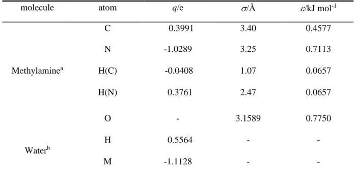
Table 1. Interaction parameters of the molecular models used.
molecule atom q/e /Å /kJ mol-1
C 0.3991 3.40 0.4577
N -1.0289 3.25 0.7113
Methylaminea H(C) -0.0408 1.07 0.0657
H(N) 0.3761 2.47 0.0657
O - 3.1589 0.7750
Waterb
H 0.5564 - -
M -1.1128 - -
aGAFF model, ref. [75], fractional charges are taken from ref. [24]
bTIP4P/2005 model, ref. [76].
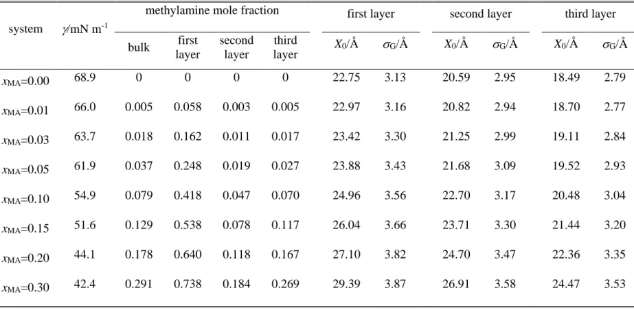
Table 2. Surface tension of the systems simulated, composition, position and width of the first three molecular layers
system /mN m-1
methylamine mole fraction first layer second layer third layer bulk first
layer
second layer
third
layer X0/Å G/Å X0/Å G/Å X0/Å G/Å
xMA=0.00 68.9 0 0 0 0 22.75 3.13 20.59 2.95 18.49 2.79
xMA=0.01 66.0 0.005 0.058 0.003 0.005 22.97 3.16 20.82 2.94 18.70 2.77
xMA=0.03 63.7 0.018 0.162 0.011 0.017 23.42 3.30 21.25 2.99 19.11 2.84
xMA=0.05 61.9 0.037 0.248 0.019 0.027 23.88 3.43 21.68 3.09 19.52 2.93
xMA=0.10 54.9 0.079 0.418 0.047 0.070 24.96 3.56 22.70 3.17 20.48 3.04
xMA=0.15 51.6 0.129 0.538 0.078 0.117 26.04 3.66 23.71 3.30 21.44 3.20
xMA=0.20 44.1 0.178 0.640 0.118 0.167 27.10 3.82 24.70 3.47 22.36 3.35
xMA=0.30 42.4 0.291 0.738 0.184 0.269 29.39 3.87 26.91 3.58 24.47 3.53
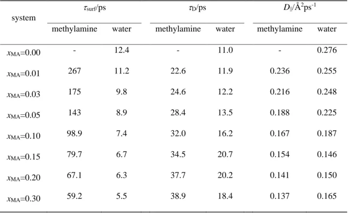
Table 3. Dynamical properties of the molecules in the surface layer
system
surf/ps D/ps D||/Å2ps-1 methylamine water methylamine water methylamine water
xMA=0.00 - 12.4 - 11.0 - 0.276
xMA=0.01 267 11.2 22.6 11.9 0.236 0.255
xMA=0.03 175 9.8 24.6 12.2 0.216 0.248
xMA=0.05 143 8.9 28.4 13.5 0.188 0.225
xMA=0.10 98.9 7.4 32.0 16.2 0.167 0.187
xMA=0.15 79.7 6.7 34.5 20.7 0.154 0.146
xMA=0.20 67.1 6.3 37.7 20.2 0.141 0.150
xMA=0.30 59.2 5.5 38.9 18.4 0.137 0.165
Figure legends
Fig. 1. Equilibrium snapshot of the surface portion of the xMA = 0.30 system. The molecules forming the first, second, and third molecular layers beneath the liquid surface are shown by blue, red, and green colours, respectively, while molecules staying beyond the third molecular layer are shown by grey colour. Lighter and darker shades of each colour represent the water and methylamine molecules, respectively. H atoms are omitted from the snapshot for clarity.
Fig.2. Comparison of the surface tension of the systems simulated (red full circles) with experimental data [87] (asterisks). The line connecting the experimental data is just a guide to the eye.
Fig. 3. Number density profile of the water (top panel) and methylamine (second panel) molecules, as well as mass density profile of the entire system (third panel) and of the first layer of the liquid phase (bottom panel) as obtained in the eight systems simulated. Grey open circles: neat water, red solid lines: xMA = 0.01 system, green dashed lines: xMA = 0.03 system, blue dash-dotted lines: xMA = 0.05 system, magenta dash-dot-dotted lines: xMA = 0. 10 system, brown dotted lines: xMA = 0.15 system, orange short dashed lines: xMA = 0.20 system, black short dash-dotted lines: xMA = 0.30 system. The inset shows the mass density profiles of the first three molecular layers beneath the liquid surface in the xMA = 0.15 system (symbols) together with their Gaussian fits (solid curves). Blue: first layer, red: second layer, green: third layer. All profiles shown are symmetrized over the two liquid-vapour interfaces present in the basic box.
Fig. 4. Methylamine mole fraction in the first (blue), second (red) and third (green) molecular layer beneath the liquid surface, as a function of the bulk liquid phase methylamine mole fraction. For reference, the straight line corresponding to the bulk phase composition itself is also shown (black solid line). The inset shows the ratio of the first layer and bulk liquid phase methylamine mole fractions as a function of the bulk liquid phase methylamine mole fraction.
The lines connecting the symbols are just guides to the eye.
Fig. 5. Mass density profile of the water (blue full circles) and methylamine (red open circles) molecules within the surface layer, together with their Gaussian fits (solid curves), as obtained in the xMA = 0.03 (top panel), xMA = 0.10 (middle panel), and xMA = 0.20 (bottom panel) systems. The inset shows the distance of the peaks of the Gaussians fitted to the water and methylamine profiles, as a function of the methylamine mole fraction in the first layer.
Fig. 6. Area distribution of the Voronoi polygons corresponding to the projections of the centres of mass of the methylamine molecules to the macroscopic plane of the surface, YZ (symbols), together with their best fits according to eq. 2 (solid curves). Red: xMA = 0.01 system, green: xMA = 0.03 system, blue: xMA = 0.05 system, magenta: xMA = 0. 10 system, black: xMA = 0.30 system.
Fig. 7. Top: definition of the local Cartesian frames fixed to the individual methylamine (left) and water (right) molecules, and that of the polar angles and of the surface normal vector, X (pointing, by our convention, to the vapor phase) in these frames. N, H, and O atoms and CH3 groups are shown by blue, white, red, and grey balls, respectively. Bottom: illustration of the splitting of the surface molecular layer to separate regions A, B, and C (see the text).
Fig. 8. Orientational maps of the methylamine molecules in the entire surface layer (first column) as well as in its separate regions C (second column), B (third column), and A (fourth column), as obtained in the xMA = 0.03 (top row), xMA = 0.10 (middel row), and xMA = 0.30 (bottom row) systems. Lighter shades correspond to higher probabilities.
Fig. 9. Orientational maps of the water molecules in the entire surface layer (first column) as well as in its separate regions C (second column), B (third column), and A (fourth column), as obtained in the xMA = 0.00 (top row), xMA = 0.03 (second row), xMA = 0.10 (third row), and xMA = 0.30 (bottom row) systems. Lighter shades correspond to higher probabilities.