C O R VI N U S E C O N O M IC S W O R K IN G P A PE R S
CEWP 06 /201 9
Production in advance versus production to order:
Equilibrium and social surplus
by Attila Tasnádi
Production in advance versus production to order:
Equilibrium and social surplus ∗
Attila Tasnádi
†Department of Mathematics, Corvinus University of Budapest, H-1093 Budapest, Fővám tér 8.
June 10, 2019
Abstract
We determine a symmetric mixed-strategy equilibrium of the production-in-advance type symmetric capacity-constrained Bertrand- Edgeworth duopoly game for the most challenging case of interme- diate capacities, which was unknown so far. Based on the obtained equilibrium we show that economic surplus within the production-to- order type environment is higher than in the respective production- in-advance type one, and therefore production-to-order should be pre- ferred to production-in-advance if the mode of production can be in- fluenced by the government.
Keywords: Price-quantity games; Bertrand-Edgeworth competition.
JEL Classification Number: D43, L13.
∗I am grateful to Iwan Bos for his very helpful remarks and suggestions. This research is granted by the Pallas Athéné Domus Sapientiae Foundation Leading Researcher Program.
†e-mail: attila.tasnadi@uni-corvinus.hu, (www.uni-corvinus.hu/~tasnadi).
1 Introduction
In one of the basic oligopoly games firms can set prices and quantities at the same time. This framework was already introduced by Shubik (1955) and referred by Maskin (1986) as the production-in-advance environment in which production takes place before sales are realized. Markets of perishable goods are usually mentioned as examples of advance production in a market.
In contrast in case of production-to-order production takes place after prices are known.
Maskin (1986) established the existence of a mixed-strategy equilibrium for the production-in-advance game under quite general conditions. Assuming unlimited capacities and linear demand, Levitan and Shubik (1978) computed the mixed-strategy equilibrium for the case of production in advance. In the same framework Gertner (1986) determined the mixed-strategy equilibrium under more general conditions. As a part of comparing the equilibrium profits under production-in-advance with that under production-to-order Tasnádi (2004, Section 4) and Tasnádi (2019) determined the equilibrium profits also for the case of unlimited capacities. Recently, Montez and Schutz (2018), as a part of a lager project on unsold inventories and exploring relations with other micro-theoretic models, determined the mixed-strategy equilibrium of the production-in-advance game and pointed out shortcomings of the previous solutions.1
In Tasnádi (2004) we showed that within the framework of a capacity- constrained Bertrand-Edgeworth duopoly the production-in-advance and the production-to-order environments result in the same profits. In obtaining this result we considered the small capacity, the intermediate capacity and the large capacity cases. Since the small capacity case has a simple solution in pure strategies (e. g. Tasnádi 2004, Section 3), while the large capacity case has been solved completely by Montez and Schutz (2018) in this paper we focus on the most challenging case of intermediate capacities for which we determine a symmetric mixed-strategy equilibrium. The latter case was only partially solved in Tasnádi (2004, Section 5), which focused only on the determination of the equilibrium profits. Furthermore, based on the derived mixed-strategy equilibrium we can show in this paper that economic surplus is higher in case of production-to-order than in case of production-in-advance.
The remainder of the paper is organized as follows: Section 2 presents the framework, Section 3 determines a symmetric mixed-strategy equilibrium and Section 4 investigates economic surplus.
1For recent theoretical results on the production in advance game we refer the reader to Bos and Vermeulen (2015) and van den Berg and Bos (2017). For related recent exper- imental results see Casaburi and Minerva (2011) and Davis (2013).
2 Preliminaries
In this section we introduce the necessary assumptions, notations and already available results.
Assumption 1. The demand curve D: R+ → R+ is strictly decreasing on [0, b], identically zero on [b,∞), continuous atb, twice continuously differen- tiable on (0, b) and concave on[0, b].
We shall denote by a the horizontal intercept of D; i.e. D(0) = a. In addition, we shall denote by P the inverse demand function.
In our model two firms set their prices and quantities simultaneously.
Assumption 2. Firms 1 and 2 have identical positive unit costs c ∈ (0, b) up to the same positive capacity constraint k. Each of them sets its price (p1, p2 ∈[0, b]) and production quantity (q1, q2 ∈[0, k]).
Throughout the paper i and j will be used to refer to the two firms; in particular, i, j ∈ {1,2}and i6=j.
We employ the efficient rationing by the low-price firm, which occurs in a market if the consumers can costlessly resell the good to each other or if the consumers have heterogeneous unit demands and the consumers having higher reservation prices are served first (for more details we refer to Vives, 1998 and Wolfstetter, 2001), to determine the demand faced by the firms.
Assumption 3. The demand faced by firm iis given by
∆i(p1, q1, p2, q2) =
D(pi) if pi < pj
qi
qi+qjD(pi) if pi =pj
(D(pi)−qj)+ if pi > pj.
Under Assumption 3 the low-price firm faces the entire demand, firms with identical prices split the demand in proportion of the firms’ quantity decisions2 and the high-price firm faces a so-called residual demand, which equals the demand minus the quantity produced by the low-price firm.
We define the firms’ profit functions as follows:
πi((p1, q1),(p2, q2)) =pimin{∆i(p1, q1, p2, q2), qi} −cqi
2The essential property of the tie-breaking rule employed in this paper is that firmi’s demand is strictly increasing in firm i’s own quantity (see also Maskin, 1986). In fact, any other tie-breaking rule satisfying the latter property does the job. Nevertheless, the tie-breaking rule specified in Assumption 3 reflects a larger visibility by consumers and a lower risk of of being out-of-stock in case of a larger production.
for both i∈ {1,2}.
Three special prices play an important role in the analysis. We definep∗ to be the price that clears the firms’ aggregate capacity from the market if such a price exists, and zero otherwise. That is,
p∗ =
D−1(2k) if D(0) >2k 0 if D(0) ≤2k.
The function
πr(p) = (p−c) (D(p)−k)
equals a firm’s residual profit whenever its opponent sells k and D(p) ≥ k.
Letp= arg maxp∈[c,b]πr(p)and π=πr(p). Clearly,p∗ andpare well defined whenever Assumptions 1 and 2 are satisfied. Finally, let p=c+π/k, that is p is the price at which a firm is indifferent between selling it entire capacity and maximizing profits on the residual demand curve.
Maskin (1986, Theorem 1) demonstrated that the production in advance game possesses an equilibrium in mixed strategies. In the following, a mixed strategy is a probability measure defined on theσ-algebra of Borel measurable sets onS = [c, b]×[0, k]. A mixed-strategy equilibrium(µ∗1, µ∗2)is determined by the following two conditions:
π1((p1, q1), µ∗2)≤π1∗, π2(µ∗1,(p2, q2))≤π2∗ (1) holds true for all (p1, q1),(p2, q2)∈S, and
π1((p∗1, q∗1), µ∗2) =π1∗, π2(µ∗1,(p∗2, q∗2)) = π2∗ (2) holds true µ∗1-almost everywhere and µ∗2-almost everywhere, where π∗1, π2∗ stand for the equilibrium profits corresponding to (µ∗1, µ∗2). In addition, it can be verified that a symmetric equilibrium in mixed strategies exists by applying Theorem 6∗ of Dasgupta and Maskin (1986).
For a strategyµletµp stand for the projection of probability measureµto the set of prices; that is, µp(B) =µ(B×[0, k])for any Borel set B ⊆ [c, b].
For a given µp we shall denote the respective cumulative distribution by F; that is, F(p) = µp([c, p]).
For the case of small capacities, i.e. p∗ ≥p, the game has a unique equi- librium in pure strategies in which the firms produce at their capacity limits and set the market-clearing price (e.g. Tasnádi, 2004, Proposition 2). The mixed-strategy equilibrium for the case of large capacities, i.e. D(c) ≤ k, has been determined recently by Montez and Schutz (2018) in which the firms charge prices above their common unit costs. Therefore, in this paper we focus on the open and most challenging case of intermediate capacities, i.e. p > max{p∗, c} for which we had established the following proposition earlier.
Proposition 1 (Tasnádi, 2004, Proposition 4). Let Assumptions 1, 2 and 3 be satisfied. If p > max{p∗, c}, then for any symmetric mixed-strategy equilibrium (µ, µ) of the production-in-advance game, we have
F(p) = µp p, p
=µ p, p
,{k}
= (p−c)k−π
p(2k−D(p)) (3) for any p∈
p, p .
3 Mixed-strategy equilibrium
We search for a symmetric mixed-strategy equilibrium in a special form by assuming that at prices p ∈ [c,bp] ⊂ [c, b] at most one quantity s(p) ∈ [0, k]
will be produced in equilibrium, where pb = inf{p∈[c, b]|µp((p, b]) = 0}.
Therefore, a mixed-strategy equilibrium can be given by the triple (p, s, Fb ).
Furthermore, we assume that sis strictly decreasing and continuously differ- entiable on [p,p). From Proposition 1 we already know thatb s(p) =k for all p∈
p, p .
Assume that(p, s, Fb )is associated with a symmetric mixed-strategy equi- librium(µ, µ). Since s and F are known for all p∈
p, p
in what follows we consider without loss of generality only prices such that p≥p. Furthermore, let f(p) =F0(p), whereF is differentiable.
Suppose that F has an atom at p. If s(p) > D(p)/2, then profits at price (p−ε, k) would be higher; a contradiction. If s(p) ≤ D(p)/2, then the expected residual demand at price p will be larger than D(p)−k, and therefore the firms’ can achieve higher profits at a price p+εthan at pricep;
a contradiction. Hence, F cannot have an atom at p. Furthermore, it can be verified that F cannot have a gap ranging from p to p+ε because then for any price in [p, p+ε] the optimal quantity of production would equalk and π1((p, q), µ)would be strictly concave on[p, p+ε]leading to a contradiction.3 We shall denote byr∗ ∈[p,p]b the unique price at which s(r∗) =D(r∗)/2 if such a price exists, otherwise we have s(p) > D(p)/2 for all p ∈ [p,p].b 4 Proceeding in a similar vein as in the proof Lemma 6 in Tasnádi (2004), it can be shown that there exists a price p0 ∈(p,p)b such thatF is even atomless on (p, p0) and that there is no gap in (p, p0). Temporarily, we assume that F
3This is just a sketch of the proof. The full proof just requires the repetition of the steps appearing in the last paragraph of the proof of Lemma 4 in Tasnádi (2004).
4This has to be shown and in the current version we are just searching for a mixed- strategy equilibrium satisfying this property.
is even atomless on (p,p). Then firmb 1’s profit equals π1((p, q), µ) = pq(1−F(p)) +p
Z p p
min
(D(p)−s(r))+, q dF(r) +
p Z p
p
min
(D(p)−k))+, q dF(r)−cq (4) for any p ∈ (p,p)b and any q ∈ [0,min{k, D(p)}], where we have already taken into account that D(p) < s(p) = q does not make sense since then the firms produce a superfluous amount for sure. Note that we cannot have q = s(p) < (D(p)−k)+ since this would result in even less profits than choosing pure-strategy(p, D(p)). Hence, in what follows we can assume that q ≥(D(p)−k)+. Therefore, (4) simplifies to
π1((p, q), µ) = pq(1−F(p)) +p Z p
p
min{D(p)−s(r), q}dF(r) +
p Z p
p
(D(p)−k)dF(r)−cq. (5)
In determining ∂π∂q1 ((p, q), µ)first let us consider the case in whichD(p)− s(p)< q, and therefore D(p)−s(r) < q for all r ∈[p, p] since s is (assumed to be) strictly decreasing. Then it follows that
∂π1
∂q ((p, q), µ) = p(1−F(p))−c. (6) Second, we consider the case in whichD(p)−s(p)> q. SinceD(p)−s(p)>
q ≥ D(p)−k =D(p)−s(p) and s is continuous and strictly decreasing on p,pb
there exists a unique r ∈ p, p
such that D(p)− s(r) = q. Then r = s−1(D(p)−q). We denote the functional relationship between q and r by r(q). Clearly, r(q) is strictly decreasing. Now (5) can be written as
π1((p, q), µ) = pq(1−F(p)) +p Z p
r(q)
qdF(r) +
p Z r(q)
p
D(p)−s(r)dF(r) +
p Z p
p
(D(p)−k)dF(r)−cq, (7)
from which we get
∂π1
∂q ((p, q), µ) = p(1−F(p)) +p Z p
r(q)
dF(r)−pqf(r(q))r0(q) +
p(D(p)−s(r(q)))f(r(q))r0(q)−c
= p(1−F(p)) +p Z p
r(q)
dF(r)−pqf(r(q))r0(q) +
pqf(r(q))r0(q)−c
= p(1−F(r(q)))−cq. (8)
Summarizing (6) and (8), we get
∂π1
∂q ((p, q), µ) =
p(1−F(p))−c if D(p)−s(p)< q,
p(1−F(r(q)))−c if D(p)−s(p)> q ≥D(p)−k.
(9) It can be verified that p(1−F (p))−c= 0 and
p
1− (p−c)k−π p(2k−D(p))
−c >0 (10)
for all p∈ p, b
\ {p}. Since F does not have an atom at price p we have π1((p, q), µ) = π
for all q∈[D(p)−k, k].
Suppose that we have (p+ ε) (1−F(p+ε))− c > 0. Then we would have s(p+ε) =k and F(p) should equal the left-hand side of (3). However, it can be verified that the expression on the left-hand side of (3) will start decreasing before achieving value 1. If we have s(p) = k even on a maximal right-open interval[p, p+ε), then from (9) it would follow that there will be a gap starting from p+ε. Since F(p+ε) <1 by the strict concavity of the profit function above the gap we can arrive to a contradiction.5
Suppose that we have(p+ε) (1−F(p+ε))−c <0. Then we would have s(p+ε) =D(p+ε)−k on an interval [p, p+ε), and therefore the residual demand starting just abovepwould be more favorable, and thus letting firm 1 achieve higher profits than π.
5This and the paragraph after the next just contains a sketch of how we can show that in case of a mixed-strategy equilibrium we have to follow the steps starting from the second paragraph from this one. However, it is not needed to demonstrate that the derived mixed strategy is a symmetric equilibrium one.
Assume that we have p(1−F(p))−c= 0for all p∈[p, r∗) resulting for any q ∈[D(p)−s(p), k]in the same profits by (9). Then
F(p) = 1− c
p (11)
for allp∈[p, r∗), and therefore the firms never produce less thanD(p)−s(p) for any p∈
p, r∗
byp(1−F(r(q)))−c >0and (9). Now from (5) and (11) we can derive s on the respective interval by solving
π =π1((p, q), µ) = pqc p+p
Z p p
(D(p)−s(r)) c r2dr+
p Z p
p
(D(p)−k)f(r)dr−cq
= pD(p)
1− c p
−pk
1− c p
−p Z p
p
s(r) c
r2dr,(12) where we have taken (9) together with our observations from this paragraph into account. Let
S(p) = Z p
p
s(r)c
r2dr (13)
for any p∈[p, r∗). Then we have
S(p) = 0 and S0(p) =s(p) c
p2 (14)
for any p∈[p, r∗). From (12) we get
S(p) =
pD(p)
1−pc
−pk
1− cp
−π
pc (15)
for any p∈ [p, r∗) from which by differentiation we obtain S0 and finally by simple rearrangements
s(p) =D0(p) p2
c2 −p c
+D(p)1 p +π
c. (16)
It can be verified that s0(p)is negative, and thus s is indeed strictly decreas- ing.
Clearly, both S and s can be extended through equations (13) and (14) for prices higher than r∗, respectively, where for p ≥ r∗ equation (12) takes
the following from
π =π1((p, q), µ) = pqc p+p
Z p r∗
s(r)c
r2dr+p Z r∗
p
(D(p)−s(r)) c r2dr+
p Z p
p
(D(p)−k)f(r)dr−cq
= pD(p) 1− c
r∗
−pk
1− c p
− p
Z r∗ p
s(r) c
r2dr+p Z p
r∗
s(r)c
r2dr. (17)
For any p≥r∗ let
Q(p) = Z p
r∗
s(r)c
r2dr. (18)
Then we have
Q(r∗) = 0 and Q0(p) =s(p) c
p2 (19)
for any p ∈ [r∗, r0), where r0 is uniquely defined by the implicit equation s(r0) =D(r0)−k. Clearly, setting prices abover0 does no make sense, since playing these pure strategies against mixed-strategy µs,F will result in less profits than pure-strategy (p, D(p)−k). From (17) we get
Q(p) =
pD(p) 1− rc∗
−pk
1− cp
−pS(r∗)−π
pc (20)
for any p ∈ [r∗, r0,) from which by differentiation we obtain Q0 and finally by simple rearrangements s(p). With a slight abuse of notation we will still denote the obtained function by s(p) on p ∈ (r∗, r0) though as it will turn out the firms will not produce at prices above r∗. These extensions will be helpful for us in the price interval [r∗, r0].
Now we will verify that having an atom at price r∗ of mass c/r∗ = 1− F(r∗)completes a symmetric mixed-strategy equilibrium. We shall denote the just completely specified price distribution by F. Assume that firm 2 plays the same mixed strategy. Then we already know that for any p ∈
p, r∗ producing an amount of q = s(p) results in π profit by Proposition 1 and the definition of s on p ∈ [p, r∗) by (14). Furthermore, for any p ∈
p, p producing less than k results in less profits then π, and for any p ∈ [p, r∗) and any quantity [D(p)−s(p), k] profits equalπ, while they are strictly less for quantities less than D(p)−s(p) by (9).
We claim that in the derived symmetric mixed-strategy equilibrium firms produce at price r∗ an amount ofs(r∗) =D(r∗)/2. Suppose that they would
produce more than D(r∗)/2. Then their will be superfluous production at price r∗, and therefore by the continuity of profits for prices below r∗ prof- its at price r∗ would be less then at prices r∗ −ε if ε is sufficiently small.
Suppose that they would produce an amount of q∗ less thanD(r∗)/2. Then π1((p, q), µs,F))is continuous at(q∗, r∗), and thereforeπ1((r∗, q∗), µs,F))< π;
a contradiction. Thus, we must have indeeds(r∗) =D(r∗)/2. By the left con- tinuity at price p∗ it follows that π1((r∗, D(r∗)/2), µs,F)) =π.
To verify that the triple (p, s, Fb ) specified in the previous paragraphs specifies a strategy of a symmetric mixed-equilibrium it remains to be shown that prices above r∗ combined with any quantity q ∈ [0, k] result in less profits than π.
The profit function of firm 1 in response to firm 2 playing the mixed strategy associated with (bp, s, F) for prices p≥r∗ equals
π1((p, q), µs,F) = pmin
D(p)−D(r∗) 2 , q
c r∗ +p
Z r∗ p
(D(p)−s(r)) c r2dr+
p Z p
p
(D(p)−k)f(r)dr−cq (21)
from which we get6
∂π1
∂q ((p, q), µ) =
( −c if D(p)−D(r2∗) < q,
prc∗ −c if D(p)−D(r2∗) > q ≥D(p)−k (22) for any p >pb=r∗. Sincepc/r∗−c >0we get that quantityq =D(p)−D(r2∗) results in the highest profit in (21) for any price p >pb=r∗.
Hence, we define the profit function of firm 1 at the best quantities for prices p≥r∗ by
π∗(p) = p
D(p)− D(r∗) 2
c r∗ +p
Z r∗ p
(D(p)−s(r)) c r2dr+
p Z p
p
(D(p)−k)f(r)dr−c
D(p)−D(r∗) 2
(23) It can be verified that π∗(p) is strictly concave, and it would be straightfor- ward to check that the derivative π∗(p)is non-positive at r∗, which unfortu- nately does not result in a manageable inequality. Therefore, we consider the
6Note that (9) is only valid for(p, q)∈(p,p)b ×[0, k], while here we need the first order condition for p >p.b
equality in (17) defining s and let us denote by πs(p) = p
Z p r∗
s(r) c
r2dr+p Z r∗
p
(D(p)−s(r)) c r2dr+
p Z p
p
(D(p)−k)f(r)dr =π (24)
for prices p ∈ [r∗, r0]. Clearly, dπs(p)/dp = 0 for any p ∈ [r∗, r0] by the definition of s, which we will utilize by considering∆(p) =
π∗(p)−πs(p) = p
D(p)− D(r∗) 2
c r∗ −c
D(p)− D(r∗) 2
−p Z p
r∗
s(r)c r2dr
=
D(p)− D(r∗) 2
p c
r∗ −c
−p Z p
r∗
s(r) c
r2dr. (25)
Then
∆0(p) = D0(p)
p c r∗ −c
+
D(p)−D(r∗) 2
c r∗ − Z p
r∗
s(r) c
r2dr−ps(p) c
p2. (26)
By substitutingr∗forpin (26) and takings(r∗) =D(r∗)/2into consideration we get ∆0(r∗) = 0, which impliesdπ∗(p)/dp= 0.
To conclude the following proposition contains our result on the mixed- strategy equilibrium of the capacity-constrained Bertrand-Edgeworth game for the case of intermediate capacities.
Proposition 2. Let Assumptions 1, 2 and 3 be satisfied. Ifp > max{p∗, c}, then a symmetric mixed-strategy equilibrium (µ, µ) is given by the following equilibrium price distribution
F(p) = µp p, p
=
0 if 0≤p < p,
(p−c)k−π
p(2k−D(p)) if p≤p < p,
1− cp if p≤p < bp=r∗, and 1 if pb=r∗ ≤p≤b
(27)
and by the ‘supply’ function s(p) given by s(p) = k for all p ∈ p, p
and determined by (16) for all p∈[p,p].b
To illustrate Proposition 2 we provide an example.
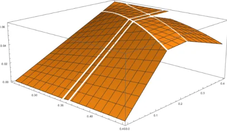
Example 1. LetD(p) = 1−p, k= 0.4and c= 0.1.
Then one can obtain that p= 0.35, π= 0.0625, p= 0.25625, s(p) = 1.625 −10p2
for all p∈[p,p], whereb pb= 0.36134060117684275, and
F(p) =
0 if 0≤p < p,
0.4p−0.12
(p−0.2)p if p≤p < p, 1−0.1p if p≤p < p,b and 1 if pb≤p≤1.
Firm 1’s profits in response to firm 2 playing its equilibrium strategy given above can be seen in Figure 1 in which prices range fromp= 0.25625to0.45 (well beyond pb = 0.36134060117684275), moreover the full quantity range from 0to 0.4is admitted.
Figure 1: Profit functionπ1((p, q), µs,F)
4 Economic surplus
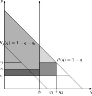
In this section we compare the production-in-advance game with the production-to-order game based on the their economic (i.e. Marshallian) sur- pluses in equilibrium, which is given by
ES(p1, q1, p2, q2) =
( Rmin{D(pj),q1+q2}
0 P(q)dq−c(q1+q2) if D(pj)> qi, Rmin{D(pi),qi}
0 P(q)dq−c(q1+q2) if D(pj)≤qi,
Figure 2: Economic surplus
where 0 ≤ pi ≤ pj ≤ b. We illustrate the economic surplus in Figure 2.
We would like to emphasize that if sales occur at the higher price, then the economic surplus is determined at the higher price.
It is well-known that for small capacities in the pure-strategy equilibrium of the production-to-order game the firms set the market-clearing price, and thus the production-to-order and the production-in-advance versions of the game have the same outcome meaning also that their economic surpluses are identical.
For large capacities in the equilibrium of the production-to-order game firms set prices equal to unit costs, while in the equilibrium of the production- in advance game firms set prices above unit costs with positive probability (see for instance, Montez and Schutz, 2018). Therefore, the economic surplus is higher in the production-to-order game than in the production-in-advance game.
For the case of intermediate capacities (i.e. p > max{p∗, c}) we know from Vives (1986) that there is only an equilibrium in nondegenerated mixed strategies with cumulative distribution function
G(p) = (p−c)k−π
(p−c) (2k−D(p)) (28)
for any p ∈ p, p
. We will rely on (28) in the proof of our next proposition stating that in case of intermediate capacities economic surplus is higher in the production-to-order game than in the production-in-advance game.
Proposition 3. Under Assumptions 1, 2, 3, p > max{p∗, c} and that the equilibrium given in Proposition 2 is played, the economic surplus is higher in the production-to-order game, then in the production-in-advance game.
Proof. First, note that the economic surplus related to the symmetric mixed- strategy equilibrium given in Proposition 2 is lower than in the case when both firms play mixed strategies F given by (27) in the production-to-order game, since then the loss in economic surplus due to both underproduction and overproduction is eliminated.
Second, since F stochastically dominates G the respective cumulative distribution function of the higher priceF2 also stochastically dominatesG2. Since the later cumulative distribution functions determine the economic surpluses the statement of the proposition holds true.
References
Bos, I., Vermeulen, D., 2015. On pure-strategy Nash equilibria in price- quantity games. Maastricht University, GSBE Research Memoranda, No. 018.
Casaburi, L., Minerva, G. A., 2011. Production in advance versus produc- tion to order: The role of downstream spatial clustering and product differentiation. Journal of Urban Economics 70, 32-46.
Dasgupta, P., Maskin, E., 1986. The existence of equilibria in discontinuous games I: Theory. Review of Economic Studies 53, 1-26.
Davis, D. D., 2013. Advance production, inventories and market power: An experimental investigation. Economic Inquiry, 51, 941-958.
Gertner, R. H., 1986. Essays in theoretical industrial organization, Ph.D.
thesis (Massachusetts Institute of Technology).
Levitan, R., Shubik, M., 1978. Duopoly with price and quantity as strategic variables. International Journal of Game Theory 7, 1-11.
Maskin, E., 1986. The existence of equilibrium with price-setting firms.
American Economic Review 76, 382-386.
Montez, J., Schutz, N., 2018. All-pay oligopolies: price competition with unobservable inventory choice. CEPR Discussion Paper 12963.
Shubik, M., 1955. A comparison of treatments of a duopoly problem (part II). Econometrica 23, 417-431.
Tasnádi, A., 2004. Production in advance versus production to order. Jour- nal of Economic Behavior and Organization 54, 191-204.
Tasnádi, A., 2019. Corrigendum to “Production in advance versus produc- tion to order.” Corvinus Economics Working Papers 2019/05.
Anita van den Berg, A., Bos, I., 2017. Collusion in a price-quantity oligopoly.
International Journal of Industrial Organization 50, 159-185.
Vives, X., 1986. Rationing rules and Bertrand-Edgeworth equilibria in large markets. Economics Letters 21, 113-116.
Vives, X., 1999. Oligopoly pricing: Old ideas and new tools (MIT Press, Cambridge MA).
Wolfstetter, E., 1999. Topics in microeconomics (Cambridge University Press, Cambridge UK).