Numerical Sensitivity Analysis on Anatomical Landmarks with regard to the Human Knee Joint
István Bíró
1, Béla M. Csizmadia
2, Gusztáv Fekete
3,41 Institute of Technology
Faculty of Engineering, University of Szeged Mars tér 7, H-6724 Szeged, Hungary biro-i@mk.u-szeged.hu
2 Institute of Mechanics and Machinery
Faculty of Mechanical Engineering, Szent István University Páter Károly utca 1, H-2100 Gödöllő, Hungary
csizmadia.bela@gek.szie.hu
3 Research Academy of Grand Health Ningbo University
Fenghua Road 818, 315000 Ningbo, China feketegusztav@nbu.edu.cn
4 Savaria Institute of Technology
Faculty of Natural and Technical Sciences, University of West Hungary Károlyi Gáspár tér 4, H-9700 Szombathely, Hungary
fekete.gusztav@ttk.nyme.hu
Abstract: For determining kinematical landmarks of the human knee joint, anatomical conventions and reference frame conventions are used by most of research teams.
Considering the irregular shapes of the femur and the tibia, the anatomical coordinate systems can be positioned with 1-2 mm and 2-4 degree position deflections. However, most of the anatomical landmarks do not appear as a dot, rather as a small surface. For this reason, the optical positioning of anatomical landmarks can only be achieved by additional 1-2 mm position deflection. It has already been proven by other authors that the application of reference frames with different positions and orientations cause significant differences in the obtained kinematics (specific anatomical landmarks and angles) of human knee joint. The goal of this research is to determine the relationship between certain anatomical landmarks and reference frames having different positions and orientations.
The investigations were carried out on cadaver knees by means of actual measurements and numerical processing.
Keywords: sensitivity analysis; anatomical landmarks; knee joint; rotation; ad/abduction
1 Introduction
In the current literature several anatomical reference frames are applied by research teams [4, 15, 16, 17]. In spite of the general intention to standardize the position and orientation of the applied reference frames, as results of invasive and noninvasive investigations, the shape of the published kinematical diagrams are quite differing. This is not only a problem in the development of surgical robot systems [27, 28], but also in kinematic-based prosthesis design. It was verified by Pennock and Clark [11] that the different position and orientation of reference frames fastened to femur and tibia yields to significant diversity of kinematical diagrams.
To solve this problem a new reference frame convention was proposed by them.
Various flexion axes have been used in the literature to describe knee joint kinematics. Among others, Most et al. [8] studied how two, widely accepted and used, flexion axes (transepicondylar axis (TEA) and the geometric center axis (GCE)) correlate with each other regarding the femoral translation and the tibial rotation. Their results suggested that kinematical calculation is sensitive to the selection of flexion axis.
Patel et al. [10] compared their own results, based on MRI images, with kinematical diagrams published by other research teams. They found similar and considerably different ones. In the study of Zavatsky et al. [14], both tibial- rotation and ad/abduction diagrams are quite different compared to the results published by other researchers. Similarly, significant difference appeared in the kinematical diagram related to the experimental study of Wilson et al. [12], who carried out tests on twelve different cadaver specimens. They assumed that the explanation of the diversity in the kinematical curves is due to the spatial orientation, the test rig design and the load.
In the presented research it will be examined how the different reference frames affect the relationship between the rotation, ad/abduction and the translation of certain anatomical landmarks on of cadaver specimens as a function of flexion angle. The investigated movement is slow knee flexion-extension, since the kinematics can be more precisely observed if the force ratios are lower than, e.g.
in case of jump-down [26]. The changes in the kinematics, related to the anatomical angles and landmarks, were determined and plotted by systematic modification of some coordinates of the anatomical landmarks.
2 Methods
2.1 Cadaver Specimens
A uniquely designed and manufactured test rig, which was also equipped with a data acquisition system to track the motion, was used to perform the experiment [7]. After the experiments the sensitivity analysis was carried out. In the presented research, eight fresh frozen human cadaveric knee specimens (5 female knees, 3 male knees; average age 56±6 years; age range 49–63 with an average BMI of 25.21±3.8) were used for the kinematical investigation.
The specimens were stored at a temperature of 0-1 C° while storage time was between 4-6 days. Each of them was manually checked to ensure the active function arc of flexion/extension (0-120°) [18]. The lengths of the knee joint specimens were approximately 40-45 cm at the center of the capsule. After resection of the knee joint specimens, the motion investigations took place within one hour. A suitable quality of capsules and bones was assured by previous radiographic images. During preparation, the skin and soft tissues were removed while the joint capsule, ligaments and muscles were left intact.
2.2 Description of the Experiment
As a first step of the kinematical investigation, coordinates of anatomical landmarks, fh, me, le, hf, tt, lm, mm were recorded on the total cadaver body lying on its back (Figure 1), where the tripods of the Polaris optical tracking system [19]
have already been attached. The accuracy of the system is 0.5 mm (volumetric:
0.25 mm RMS).
Figure 1
Anatomical landmarks on femur and tibia (right side) [6]
The anatomical landmarks are:
- Coordinates of centre of the femoral head (fh), - Coordinates of medial and lateral epicondyles (me, le),
- Coordinates of apex of the head of the fibula (hf), - Coordinates of prominence of the tibial tuberosity (tt),
- Coordinates of distal apex of the lateral and medial malleolus (lm, mm).
In addition, the following points must be defined:
- The origin (Ot) of the anatomical coordinate system, which is the midpoint of the junction-line between the medial (me) and lateral (le) epicondyles, - The yt axis of the coordinate system, which is the line between the origin
and the center of the femoral head (fh), pointing upward with positive direction,
- The xt axis of the coordinate system is perpendicular to the quasi-coronal plane, defined by the three anatomical points (hf, me, le). It has positive direction to the anterior plane,
- The zt axis of the coordinate system is mutually perpendicular to the xt and the yt axis with positive direction to the right.
Figure 2 represents these landmarks and points.
Figure 2
Anatomical landmarks on femur and tibia (right side) [6]
First of all, the coordinates of medial and lateral epicondyles (me, le) were pinpointed and recorded in the absolute coordinate system (XYZ) (Figure 3).
Figure 3
Pinpointing and recording anatomical landmarks on femur (right side)
Then by the use of a simple transformation (eq. (1) and eq. (2)) [25], the registered points (le, me, fh) can be transferred into the coordinate-system attached to the femur (Xfe-Yfe-Zfe) (Figure 4):
r
a
T x
x
1
(1)
1 1 0 0 0
1
1
33 32 31
23 22 21
13 12 11
z y x
Z Y X
T T T
T T T
T T T
Z Y X
O O O
(2)
Figure
Pinpointing and recording anatomical landmarks on femur (right side)
This step was followed by circularly moving the thigh in order to determine the center of the femoral head (fh) in the absolute coordinate system (XYZ) (Figure 4). After this, the same transformation (eq. (1) and eq. (2)) was carried out to transform the femoral head (fh) into the Xfe-Yfe-Zfe coordinate system.
Four screws were attached to the femur, which represent the reference points.
These reference points are pinpointed and recorded in the absolute coordinate system (XYZ) (Figure 5a). Then, they were similarly transformed into the Xfe-Yfe-Zfe coordinate system (Fig. 5b).
Figure 5a and Figure 5b
Pinpointing and transforming reference points on femur (right side)
Closely the same procedure must be carried out on the tibia as well. The coordinates of the head of the fibula (hf), the tibial tuberosity (tt) and the lateral and medial malleolus (mm, lm) were pinpointed and recorded in the absolute coordinate system (XYZ) (Figure 6).
Figure 6
Pinpointing anatomical landmarks on tibia in the absolute (XYZ) coordinate system (right side) Then again, by the use of a simple transformation (eq. (1) and eq. (2)) [25], the registered points (hf, tt, lm, mm) can be transferred into the coordinate-system attached to the tibia (Xte-Yte-Zte) (Figure 7):
Figure 7
Pinpointing anatomical landmarks on tibia in the relative (Xte, Yte, Zte) coordinate system (right side)
The identification of the landmarks on the intact cadaver knee was followed by the resection of the cadaver specimens (Fig. 8). The flexion/extension movement on the cadaver specimens were carried out in the test rig.
Figure 8
Cadaver specimen with two positioning sensors
During the measurement, the following conditions were kept: a) the knee joint carried out unconstrained motion; b) the test rig is equipped with a Polaris optical tracking system [19], which allows motion data acquisition under flexion/extension movement with a configuration of moving (rotating) tibia and fixed femur; c) motion data can be recorded in any arbitrary flexed position; d) the angular velocity of tibia related to femur is adjustable; e) the acting forces of the knee joint can be measured during flexion/extension; f) the tibia starts its motion by moving downwards from the extended position. The tibia is loaded in the sagittal plane of the knee joint. The loading force, acting on the end of tibia, enables the unconstrained flexion/extension motion while the test rig assures at least 120 degrees in flexion. Each specimen was manually flexed and extended five times before its actual installation into the test rig. Two plastic beams were fixed on both sides of the specimen. A rubber strip, representing the muscle model, was fixed to the quadriceps tendon of the cadaver knee joint. The trend of the quadriceps force function, regarding the magnitude of the force, is approximately linear up to a 70-80 degree of flexion angle [21, 22, 23, 24]. For this reason, a rubber strip was used to model the muscle, its characteristic was tested and showed linear behavior in the applied interval.
Anatomical conventions, reference frame convention and joint system convention of the VAKHUM project [6] were applied in the presented research. These conventions are based on current international standards (e.g. from the International Society of Biomechanics).
The main steps of the measurement are the followings [1, 2, 3, 7]:
Table 1
Steps of the experiment protocol
Description
1 During the preparation of the cadaver knee joint, 4 + 4 screws are to be fixed into the femur and tibia. Screw heads are reference points in the course of measurement.
2 The position of the screw heads (as reference points) have to be recorded in the reference frames of the sensors.
3 The position sensors have to be attached to the lying cadaver body (femur and tibia).
4 The position of the anatomical landmarks (le, me, tt, hf, mm, lm) have to be recorded in the reference frames of the sensors.
5 The position of anatomical landmark fh in absolute coordinate-system of Polaris optical tracking system (pelvis is immovable) is to be determined by manually constrained thigh circle.
6 After the removal of the sensors, the resection has to be performed on the knee joint capsule.
7 The capsule has to be fixed into the test rig (Fig. 2).
8 The sensors have to be re-attached to both sides of the capsule (femur and tibia), obviously in a different position compared to the previous ones.
9 Data acquisition regarding the position of the 4 + 4 screw heads has to be repeated.
10 The position data of the anatomical landmarks (le, me, tt) in the coordinate-systems of sensors (in a modified position) has to be recorded.
11 The flexion/extension data of the knee joint can be continuously recorded by the sensors attached to the tibia and femur.
2.3 Description of the Parameters and Coordination Frames
Motion components of the knee joint were calculated according to the convention of Pennock and Clark [11]. The calculation is based on a three-cylindrical mechanism using Denavit-Hartenberg [5] parameters. In order to plot the kinematical diagrams, several reference frames were used such as the absolute reference frame of the Polaris optical tracking system, the reference frames of the sensors attached to the femur and the tibia, and the anatomical reference frames attached to the femur and the tibia (Fig. 8 and Fig. 9).
With the object to create the determining matrix-equation, the required anatomical landmarks on the femur and the tibia Pi (i=1,2,…..,7) are the following: femoral head (fh): P1 (X1,Y1,Z1), medial epycondylus (me): P2 (X2,Y2,Z2), lateral epycondylus (le): P3 (X3,Y3,Z3), lateral malleolus (lm): P4 (X4,Y4,Z4), medial malleolus (mm): P5 (X5,Y5,Z5), tibial tuberosity (tt): P6 (X6,Y6,Z6), apex of the head of the fibula (hf): P7 (X7,Y7,Z7). These points are appointed on Fig. 8 and Fig. 9.
Figure 8
Position of anatomical reference frame XoYoZo joined to femur in reference frame fs (cadaver lying on his back, investigated right leg, view from medial side)
Figure 9
Position of anatomical reference frame xsyszs and X3Y3Z3 joined to tibia in reference frame ts (cadaver lying on his back, investigated right leg, view from medial side)
The mathematical relationship between the applied coordinate-systems can be described by the following matrix-equation:
A B C1D1
E .(3) where:
[A]: fourth-order transformation matrix between reference frame ts (attached to tibia sensor) and anatomical reference frame X3Y3Z3 fixed to tibia:
1 0 0 0
42 42 41
32 32 31
22 22 21
13 12 11
A A A
A A A
A A A
A A A
.
(4) Elements of matrix [A] and vector operations-notations to determine them:
2 4 5 2 4 5 2 4 5
3 (X X ) (Y Y) (Z Z )
N
2 4 7 2 4 7 2 4 7
4
( X X ) ( Y Y ) ( Z Z )
N
2 5 4 6 2 5 4 6 2 5 4 6
5
( 2 X X X ) ( 2 Y Y Y ) ( 2 Z Z Z )
N
4 3 4
3
4 7 4 5 4 5 4 7 23
4 3 4
3
4 7 4 5 4 5 4 7 22
4 3 4
3
4 7 4 5 4 5 4 7 21
) )(
( ) )(
(
) )(
( ) )(
(
) )(
( ) )(
(
N N N
N
Y Y X X Y Y X A X
N N N
N
Z Z X X Z Z X A X
N N N
N
Z Z Y Y Z Z Y A Y
5 4 3
5 4 6 5
4 6 13
5 4 3
5 4 6 5
4 6 12
5 4 3
5 4 6 5
4 6 11
) 2
( ) 2
(
) 2
( ) 2
(
) 2
( ) 2
(
N N N
Y Y Y X
X A X
N N N
Z Z Z X
X A X
N N N
Z Z Z Y
Y A Y
5 2 4 2 3
5 4 6 5
4 6
5 4 6 5
4 6
33
5 2 4 2 3
5 4 6 5
4 6
5 4 6 5
4 6
32
5 2 4 2 3
5 4 6 5
4 6
5 4 6 5
4 6
31
)) 2
( ) 2
((
) ))(
2 ( ) 2
((
)) 2
( ) 2
((
)) 2
( ) 2
((
)) 2
( ) 2
((
)) 2
( ) 2
((
N N N
Z Z Z X
X X
Z Z Z Y
Y Y A
N N N
Y Y Y X
X X
Z Z Z Y
Y Y A
N N N
Y Y Y X
X X
Z Z Z X
X X A
( )2 );1 2(
);1 2(
; 1
; 42 43 4 5 4 5 4 5
41 A A X X Y Y Z Z
A
[B]: fourth-order transformation matrix between the absolute reference frame and reference frame ts attached to tibia sensor:
1 0 0 0
42 42 41
32 32 31
22 22 21
13 12 11
B B B
B B B
B B B
B B B
B .
(5) Elements of matrix [B] in which OXts, OYts, OZts, are the coordinates of the origin of reference frame attached to tibia sensor in the absolute reference frame and Ψts, Θts, Φts are Euler-angles between the same reference frames. These data were measured by Polaris optical tracking system.
1 0 cos cos sin sin cos cos sin cos sin cos sin sin
0 cos sin sin sin sin cos cos cos sin sin sin cos
0 sin sin
cos cos
cos
1 0 0 0
43 42 41
33 32 31
23 22 21
13 12 11
Zts Yts
Xts
ts ts ts ts ts ts ts ts ts ts ts ts
ts ts ts ts ts ts ts ts ts ts ts ts
ts ts
ts ts
ts
O O
O B
B B
B B B
B B B
B B B
[C]: fourth-order transformation matrix between the absolute reference frame and reference frame fs attached to femur sensor:
1 0 0 0
42 42 41
32 32 31
22 22 21
13 12 11
C C C
C C C
C C C
C C C
C .
(6) Elements of matrix [C] in which OXfs, OYfs, OZfs, are the coordinates of the origin of reference frame attached to femur sensor in the absolute reference frame and Ψfs, Θfs, Φfs are Euler-angles between the same reference frames. These data were measured by Polaris optical tracking system.
1 0 cos cos sin sin cos cos sin cos sin cos sin sin
0 cos sin sin sin sin cos cos cos sin sin sin cos
0 sin sin
cos cos
cos
1 0 0 0
43 42 41
33 32 31
23 22 21
13 12 11
Zfs Yfs
Xfs
fs fs fs fs fs fs fs fs fs fs fs fs
fs fs fs fs fs fs fs fs fs fs fs fs
fs fs
fs fs
fs
O O
O C
C C
C C C
C C C
C C C
[D]: fourth-order transformation matrix between reference frame fs (attached to femur sensor) and anatomical reference frame XoYoZo fixed to femur:
1 0 0 0
42 42 41
32 32 31
22 22 21
13 12 11
D D D
D D D
D D D
D D D
D .
(7)
Elements of matrix [D] and vector operations-notations to determine them:
2 1 3 2 2 1 3 2 2 1 3 2
1 (X X 2X ) (Y Y 2Y) (Z Z 2Z )
N
1 1 3 2 1
1 3 2 1
1 3 2 13
12 11
2 2
2
N Z Z
; Z N
Y Y
; Y N
X X D X
; D
; D
2 2 3 2 2 3 2 2 3
2 (X X ) (Y Y) (Z Z )
N
2 1
2 3 1 3 2 1 3 2 2 3 23
2 1
2 3 1 3 2 1 3 2 2 3 22
2 1
2 3 1 3 2 1 3 2 2 3 21
) )(
2 (
) 2 )(
(
) )(
2 (
) 2 )(
(
) )(
2 (
) 2 )(
(
N N
Y Y X X X Y Y Y X D X
N N
Z Z X X X Z Z Z X D X
N N
Z Z Y Y Y Z Z Z Y D Y
2 2 1
1 3 2 2 3 1 3 2 1 3 2 2 3
2 2 1
2 3 1 3 2 1 3 2 2 3 1 3 2 33
2 2 1
1 3 2 2 3 1 3 2 1 3 2 2 3
2 2 1
2 3 1 3 2 1 3 2 2 3 1 3 2 32
2 2 1
1 3 2 2 3 1 3 2 1 3 2 2 3
2 2 1
2 3 1 3 2 1 3 2 2 3 1 3 2 31
) 2 ))(
)(
2 (
) 2 )(
((
)) )(
2 (
) 2 )(
( )(
2 (
) 2 ))(
)(
2 (
) 2 )(
((
)) )(
2 (
) 2 )(
)((
2 (
) 2 ))(
)(
2 (
) 2 )(
((
)) )(
2 (
) 2 )(
)((
2 (
N N
Y Y Y Z Z Y Y Y Z Z Z Y Y
N N
Z Z X X X Z Z Z X X X X D X
N N
Z Z Z Z Z Y Y Y Z Z Z Y Y
N N
Y Y X X X Y Y Y X X X X D X
N N
Z Z Z Z Z X X X Z Z Z X X
N N
Y Y X X X Y Y Y X X Y Y D Y
( )2 );1 2(
);1 2(
; 1
; 42 43 2 3 2 3 2 3
41 D D X X Y Y Z Z
D
[E]: fourth-order transformation matrix between reference frame X3Y3Z3 and reference frame XoYoZo.
1 0 0 0
42 42 41
32 32 31
22 22 21
13 12 11
E E E
E E E
E E E
E E E
E .
(8) Elements of matrix [E] (Θ1, Θ2, Θ3, d1, d2, d3, are the obtained kinematical parameters of human knee joint).
3 1 3
2 1
11cos cos cos sin sin
E ;
3 1
3 2
1
12sin cos cos cos sin
E ;
3 2
13 sin cos
E ;
3 1
3 2
1
21cos cos sin sin cos
E ;
3 1
3 2 1
22 sin cos sin cos cos
E ;
3 2
23 sin sin
E ;
2 1
31
cos sin
E
; E32 sin1sin2; E33cos2;1 2 2 1 3
41d cos sin d sin
E ;
1 2
2 1 3
42 d sin sin d cos
E ;
1 2 3
43 d cos d
E .
Elements of matrix [E] contain the six kinematical parameters of human knee joint complying with the constraint conditions of the three-cylindrical mechanism model, which has been described by the Denavit-Hartenberg (later on HD) parameters – was used (Fig. 10). By the use of the HD parameters, the variables are reduced from six to four (Θi, di, li, αi). These parameters fit well to the geometrical particularities of the applicable bodies and constraints [[5]].
Figure 10
Human knee joint model in extended position [5]
In Fig. 10, the HD coordinates can be seen. The parameters of αi, li, (i=1,2,3) can be adjusted optionally according to the special geometry of knee joint. On the basis of the published recommendations [[11]] the following data is supported as a correct setting: α1=α2=90o, α3=0o, l1=l2=l3=0. The application of the model enables the calculation of the following quantities (Fig. 10):
Θ1 – flexion, plotted as 0 degree, Θ2 – ad/abduction, plotted as 90 degree, Θ3 – rotation of the tibia, plotted as 0 degree, d1, d2, d3 – moving on accordant axes.
lm, mm
2.4 Description of the Sensitivity Analysis
The aim of the numerical sensitivity analysis is to describe how the rotation, ad/abduction and translation of the (fh, me, le, lm, mm, tt, hf) depend on the position of the anatomical points therefore it also depends on the anatomical peculiarity of each subject.
This is also interpreted by the coordinate systems since they are defined by these anatomical points. The anatomical coordinate systems can be defined within a few mm including the deviation or error of the irregular form of the femur and tibia, and their anatomical peculiarities as well.
The detection of the position of the centre of femoral head (P1), the apex of the head of the fibula (P7) and prominence of the tibial tuberosity (P6) cause only small angular deviation, since these anatomical landmarks are located relatively far from the origins of the coordinate systems (Fig. 3 and Fig. 4). The origins of the coordinate-systems are determined between the epicondyles and the apices of the lateral and medial malleolus, therefore the effect of position deflection is quite significant on the position and the orientation of the reference frame.
The numerical sensitivity analysis was carried out by a matrix-equation including 21 position coordinates of seven anatomical landmarks (three on the femur and four on the tibia). The position and orientation of the tibia related to the femur was changing step-by-step as a function of flexion angle.
At each step the position and the orientation of the tibia sensor changes therefore each time step another equation-system is generated.
By solving these equation-systems, three rotational and three translational parameters can be obtained, which determine the position and orientation of the tibia related to the femur.
As a first step of sensitivity analysis, the positions of epicondyles (points P2 and P3) were modified step-by-step (±2 mm) in the quasi-transverse plane in the opposite direction (cadaver lying on his back, extended position). In the second phase the positions of apices of the lateral and medial malleolus (points P4 and P5) were modified step-by-step (±2 mm) in quasi-transverse plane in the opposite direction as well. Difference compared to the basic functions (bold curve) are plotted in Fig. 10 and Fig. 11. The basis function contains some error since it was calculated from measured data.
3 Results
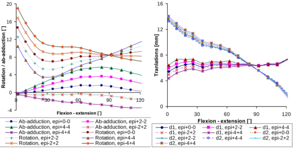
As we look at the group of curves created by systematic step-by-step position modification of the epicondyles, it is observable that in the first phase of flexion (until 40 degrees) the rotation-flexion curves are shifted parallel, while over 40 degrees their slopes are significantly different. The ad/abduction-flexion curves start from almost the same point, but the slope and the shape of the functions are quite divergent. The effect of the position modification of the epicondyles is negligible on the displacement components of the knee joint model (Fig. 11abc).
In case of systematic step-by-step position modification of the lateral and medial malleolus, the rotation-flexion curves are shifted parallel moreover the ad/abduction-flexion curves are nearly unchanged. The medio-lateral and antero- posterior translational curves are shifted parallel furthermore the proximal-distal translation along the tibial axis is quite unchanged (Fig. 12abc).
It is also apparent that the shapes of investigated kinematical diagrams depend considerably on the position and orientation of the reference frames fastened to femur and tibia. The shape and position of the kinematical curves were modified due to the different recorded position of the anatomical landmarks.
By the obtained new information, the kinematical results, carried out on different cadaver subjects, becomes comparable. Rotation-flexion and ad/abduction-flexion diagrams (Fig. 11a) are similar to the ones found in the literature.
-4 0 4 8 12 16 20
0 30 60 90 120
Flexion - extension [˚]
Rotation / ab-adduction [˚]
Ab-adduction, epi+0-0 Ab-adduction, epi+2-2 Ab-adduction, epi+4-4 Ab-adduction, epi-2+2 Ab-adduction, epi-4+4 Rotation, epi+0-0 Rotation, epi+2-2 Rotation, epi+4-4 Rotation, epi-2+2 Rotation, epi-4+4
0 4 8 12 16
0 30 60 90 120
Flexion - extension [˚]
Tranlations [mm]
d1, epi+0-0 d1, epi+2-2 d1, epi+4-4 d1, epi-2+2 d1, epi-4+4 d2, epi+0-0 d2, epi+2-2 d2, epi+4-4 d2, epi-2+2 d2, epi-4+4
Figure 11a and Figure 11b Coordinate modification of the epycondyles
Every single curve was plotted after systematic modification of the epicondyles position in the femur quasi-transverse plane.
424.5 425 425.5 426 426.5 427 427.5 428 428.5
0 30 60 90 120
Flexion - extension [˚]
Tranlation [mm]
d3, epi+0-0 d3, epi+2-2 d3, epi+4-4 d3, epi-2+2 d3, epi-4+4
Figure 11c
Coordinate modification of the epycondyles
The curves point out well how the rotation-flexion and the ad/abduction-flexion diagrams depend on the position of the epicondyles. The modification of the condyle peaks did not influence significantly the shape of the translational diagrams (Fig. 11b-c).
As a second step, the effect of the coordinate modification of the malleolus is considered. As it is seen in Fig. 12a, the rotation-flexion curves are shifted parallel, due to the systematic position modification of the lateral and medial malleolus in the tibia quasi-transverse plane.
0 4 8 12 16 20
0 30 60 90 120
Flexion - extension [˚]
Rotation [˚]
Rotation, mal+0-0 Rotation, mal+2-2 Rotation, mal+4-4 Rotation, mal-2+2 Rotation, mal-4+4
0 4 8 12 16 20
0 30 60 90 120
Flexion - extension [˚]
Translations [mm]
d1, mal+0-0 d1, mal+2-2 d1, mal+4-4 d1, mal-2+2 d1, mal-4+4 d2, mal+0-0 d2, mal+2-2 d2, mal+4-4 d2, mal-2+2 d2, mal-4+4
Figure 12a and Figure 12b Coordinate modification of the malleolus
Translational curves d1 and d2 are shifted parallel (Fig. 12b), while the ad/abduction -flexion curves (Fig. 12c) and the curves d3 are nearly the same (Fig.
11c).
-1 -0.5 0 0.5 1 1.5 2 2.5
0 30 60 90 120
Flexion - extension [˚]
Ab-adduction [˚]
Ab-adduction, mal+0-0 Ab-adduction, mal+2-2 Ab-adduction, mal+4-4 Ab-adduction, mal-2+2 Ab-adduction, mal-4+4
Figure 12c
Coordinate modification of the malleolus
On the basis of the obtained groups of curves, the analysis of other kinematical diagrams becomes possible regarding the anatomical features of the investigated person and the accuracy/inaccuracy of positioning of anatomical landmarks.
Conclusions
By the obtained new information, the kinematical results, carried out on different cadaver subjects, becomes comparable. Rotation-flexion and ad/abduction-flexion diagrams are similar to the ones found in the literature, nevertheless the presented measurement and processing methods, together with the sensitivity analysis, can quantitatively show how kinematical parameters of the knee joint (ad/abduction, rotation) are influenced by the coordinate systems fixed to the femur and tibia under flexion-extension. In this demonstration, every single curve was plotted after systematic modification of the epicondyles position in the femur quasi- transverse plane, thus the curves point out well how the rotation-flexion and the ad/abduction-flexion diagrams depend on the position of the epicondyles.The modification of the condyle peaks did not influence significantly the shape of the translational diagrams. As it is demonstrated, the rotation-flexion curves are shifted parallel, due to the systematic position modification of the lateral and medial malleolus in the tibia quasi-transverse plane. Translational curves d1 and d2 are also shifted parallel. The ad/abduction-flexion curves and the curves d3 are nearly the same. On the basis of the obtained groups of curves, the analysis of other kinematical diagrams becomes possible regarding the anatomical features of the investigated person and the accuracy/inaccuracy of positioning of anatomical landmarks.
Acknowledgements
The presented research was supported by University of Szeged, Szent István University, University of West Hungary and by the Zhejiang Social Science Program – Zhi Jiang youth project (Project number: 16ZJQN021YB).
References
[1] Bíró, I., and Csizmadia, B. M.: Translational Motions in Human Knee Joint Model, Review of Faculty of Engineering, Analecta Technica Szegedinensia, 2-3: 23-29 (2010)
[2] Bíró, I., Csizmadia, B. M., Katona, G.: New Approximation of Kinematical Analysis of Human Knee Joint, Bulletin of Szent István University, 330-338 (2008)
[3] Bíró, I., Csizmadia, B. M., Krakovits, G., Véha, A.: Sensitivity Investigation of Three-Cylinder Model of Human Knee Joint, IUTAM Symposium on Dynamics Modelling and Interaction Control in Virtual and Real Environments, Book Series 30: 177-184, Budapest, 7-11 June (2010) [4] Bull, A. M. J., Amis, A. A.: Knee Joint Motion: Description and
Measurement,” Proceedings of the Institution of Mechanical Engineers, Part H: Journal of Engineering in Medicine, 212: 357-372 (1998)
[5] Denavit, J., Hartenberg, R. S.: A Kinematic Notation for Lower-Pair Mechanism Based on Matrices, ASME Journal of Applied Mechanics, 22:
215-221 (1955)
[6] http://www.ulb.ac.be/project/vakhum
[7] Katona, G., Csizmadia, B. M., Bíró, I., Andrónyi, K., Krakovits, G.: Motion Analysis of Human Cadaver Knee-Joints using Anatomical Coordinate System, Biomechanica Hungarica, 1: 93-100 (2009)
[8] Most, E., Axe, J., Rubash, H., Li, G.: Sensitivity of the Knee Joint Kinematics Calculation to Selection of Flexion Axes, Journal of Biomechanics 37: 1743-1748 (2004)
[9] Northern Digital Inc.: Polaris Optical Tracking System, Application Programmer’s Interface Guide (1999)
[10] Patel, V. V., Hall, K., Ries, M., Lotz, J., Ozhinsky, E., Lindsey, C., Lu, Y., Majumdar, S.: A Three-Dimensional MRI Analysis of Knee Kinematics, Journal of Orthopaedic Research 22: 283-292 (2004)
[11] Pennock, G. R., Clark, K. J.: An Anatomy-based Coordinate System for the Description of the Kinematic Displacements in the Human Knee, Journal of Biomechanics 23: 1209-1218 (1990)
[12] Wilson, D. R., Feikes, J. D., Zavatsky, A. B., O’Connor, J. J.: The Components of Passive Knee Movement are Coupled to Flexion Angle, Journal of Biomechanics 33: 465-473 (2000)
[13] Wu, G., Canavagh, P. R., ISB Recommendation for Standardization in the Reporting of Kinematic Data, Journal of Biomechanics, 28: 1257-1261 (1995)
[14] Zavatsky, B., Oppold, P. T., Price, A. J.: Simultaneous In Vitro Measurement of Patellofemoral Kinematics and Forces, Journal of Biomechanical Engineering, 126: 351-356 (2004)
[15] Stagni, R., Fantozzi, S., Capello A.: Propagation of Anatomical Landmark Displacement to Knee Kinematics: Performance of Single and Double Calibration, Gait and Posture, 24: 137-141 (2006)
[16] Rapoff, A. J., Johnson, W. M., Venkataraman S., Transverse Plane Shear Test Fixture for Total Knee System, Experimental Techniques, 27: 37-39 (2003)
[17] Fekete, G., De Baets, P., Wahab, M. A., Csizmadia M. B., Katona, G., Vanegas-Useche V. L., Solanilla, J. A.: Sliding-Rolling Ratio during Deep Squat with regard to Different Knee Prostheses, Acta Polytechnica Hungarica, 9 (5): 5-24 (2012)
[18] Freeman, M. A. R.: How the Knee Moves. Current Orthopaedics, 15: 444- 450 (2001)
[19] http://www.ndigital.com/medical/polarisfamily-techspecs.php
[20] Singerman, R., Berilla, J., Archdeacon, M., Peyser, A.: In Vitro Forces in the Normal and Cruciate Deficient Knee during Simulated Squatting Motion. Journal of Biomechanical Engineering, 121: 234-242 (1999) [21] Cohen, Z. A., Roglic, H., Grelsamer, R. P., Henry, J. H., Levine, W. N.,
Mow, V. C., Ateshian, G. A.: Patellofemoral Stresses during Open and Closed Kinetic Chain Exercises – An Analysis using Computer Simulation.
The American Journal of Sports Medicine, 29: 480-487 (2001)
[22] Mason, J. J., Leszko, F., Johnson, T., Komistek, R. D.: Patellofemoral Joint Forces. Journal of Biomechanics, 41: 2337-2348 (2008)
[23] Fekete, G.: Fundamental Questions on the Patello- and Tibiofemoral Knee Joint: Modelling Methods related to Patello- and Tibiofemoral Kinetics and Sliding-Rolling Ratio under Squat Movement. Scholar’s Press, Saarbrücken, Germany, 2013
[24] Fekete, G., Csizmadia, B. M., Wahab, M. A., De Baets, P., Vanegas- Useche, L. V., Bíró, I.: Patellofemoral Model of the Knee Joint under Non- Standard Squatting. Dyna, 81 (183): 60-67 (2014)
[25] Bíró, I., Fekete, G.: Approximate Method for Determining the Axis of Finite Rotation of Human Knee Joint, Acta Polytechnica Hungarica, 11 (9):
61-74 (2014)
[26] Melińska, A., Czamara, A., Szuba, L., Będziński, R., Klempous, R.:
Balance Assessment during the Landing Phase of Jump-Down in Healthy Men and Male Patients after Anterior Cruciate Ligament Reconstruction.
Acta Polytechnica Hungarica, 12 (6): 77-91 (2015)
[27] Takács, Á., Kovács, L., Rudas, I. J., Precup, R-E., Haidegger, T.: Models for Force Control in Telesurgical Robot Systems. Acta Polytechnica Hungarica, 12 (8): 95-114 (2015)
[28] Hošovský, A., Piteľ, J., Židek, K., Tóthová, M., Sárosi, J., Cveticanin, L.:
Dynamic Characterization and Simulation of Two-Link Soft Robot Arm with Pneumatic Muscles. Mechanism and Machine Theory, 103: 98-116 (2016)