Deep learning in static, metric-based bug prediction
Rudolf Ferenc
a,*, D enes B an
a, Tam as Gr osz
b,c, Tibor Gyim othy
a,caDepartment of Software Engineering, University of Szeged, Hungary
bDepartment of Computer Algorithms and Artificial Intelligence, University of Szeged, Hungary
cMTA-SZTE Research Group on Artificial Intelligence, Szeged, Hungary
A R T I C L E I N F O Keywords:
Neural networks Deep learning Bug prediction Code metrics
A B S T R A C T
Our increasing reliance on software products and the amount of money we spend on creating and maintaining them makes it crucial tofind bugs as early and as easily as possible. At the same time, it is not enough to know that we should be paying more attention to bugs;finding them must become a quick and seamless process in order to be actually used by developers. Our proposal is to revitalize static source code metrics–among the most easily calculable, while still meaningful predictors–and combine them with deep learning–among the most promising and generalizable prediction techniques–toflag suspicious code segments at the class level. In this paper, we show a detailed methodology of how we adapted deep neural networks to bug prediction, applied them to a large bug dataset (containing 8780 bugged and 38,838 not bugged Java classes), and compared them to multiple
“traditional”algorithms. We demonstrate that deep learning with static metrics can indeed boost prediction ac- curacies. Our best model has an F-measure of 53.59%, which increases to 55.27% for the best ensemble model containing a deep learning component. Additionally, another experiment suggests that these values could improve even further with more data points. We also open-source our experimental Python framework to help other re- searchers replicate ourfindings.
1. Introduction
Our society’s ever increasing reliance on software products puts pressure on developers that is close to unsustainable. With fast idea-to- market times, common overtime issues, and global competition, soft- ware faults–or bugs, as they are more commonly referred to–are easy to make, but hard and costly tofix [1]. Moreover, this cost increases pro- portionately with the time of discovery, so the earlier we can catch them, the better. Considering the scale of today’s source code, however, this requires more automated support than ever. Even if we are not on the level of intelligentfixes or perfect recall yet, narrowing down the po- tential candidates or highlighting points of interest can be crucial for engineers to be able to keep up with demand.
How these candidates are produced is still a heavily researched area, though. Dynamic or symbolic analyses could provide much more exact matches, but they also require more time and resources per every piece of software under consideration. This is the main reason we are aiming to restrict our necessary analysis techniques to static only. Another issue can be insufficient data for generalizability, which is why we are using the largest unified class level dataset [2] we are aware of.
With the above constraints in place, most of the remaining research focuses on“traditional”machine learning approaches like decision trees, Bayesian models or Support Vector Machines for example. We, on the other hand, focus on deep learning and how it can be applicable to the same problem, since it already showed promising general use in other areas.
Deep learning is a new and very successful area in machine learning;
the name stems from the fact that it applies deep neural networks (DNNs). These deep networks differ from previously used artificial neural networks in one key aspect, namely that they contain many hidden layers. Unfortunately, with these deep structures we have to face the fact that the traditional training algorithm encounters difficulties (“vanishing gradient effect”) and fails to train good models. As a solution to this problem, several new algorithms and modifications have been proposed over the years. Of these, we opted for one of the simplest ones, the so called deep rectifier network [3]. With a simple modification to the activation function, the DNN can be trained without any further changes using the standard stochastic gradient descent (SGD) algorithm.
Our plan was to take the above mentioned bug dataset and use it to compare the performance of DNNs to other, more traditional machine
* Corresponding author. H-6720, Szeged, Dugonics ter 13, Hungary.
E-mail addresses: ferenc@inf.u-szeged.hu (R. Ferenc), zealot@inf.u-szeged.hu (D. Ban), groszt@inf.u-szeged.hu (T. Grosz), gyimothy@inf.u-szeged.hu (T. Gyimothy).
Contents lists available atScienceDirect
Array
journal homepage:www.elsevier.com/journals/array/2590-0056/open-access-journal
https://doi.org/10.1016/j.array.2020.100021
Received 16 December 2019; Received in revised form 16 February 2020; Accepted 23 February 2020 Available online 30 March 2020
2590-0056/©2020 The Authors. Published by Elsevier Inc. This is an open access article under the CC BY license (http://creativecommons.org/licenses/by/4.0/).
Array 6 (2020) 100021
learning techniques within the domain of bug prediction–specifically, bug prediction from static source code metrics. We emphasize the interdisciplinary aspect of this experiment by thoroughly detailing every step we took on our way to training our optimal model, including the possible data preprocessing, parameterfine-tuning, and further exami- nations regarding current or future expectations. Consequently, the coming sections could be a useful tool for static analysts not familiar with deep learning, while the nature and quantity of the data–along with the conclusions we can draw from them–could provide new insights for machine learning practitioners as well.
Our best deep learning model achieved an F-measure of 53.59% using a dynamically updated learning rate on the quite imbalanced bug dataset, which contains 8780 (18%) bugged and 38,838 (82%) not bugged Java classes. The only single approach capable of outperforming it was a random forest classifier with an improvement of 0.12%, while an ensemble model combining these two reached an F-measure of 55.27%.
Additionally, a separate experiment suggests that these deep learning results could increase even further with more data points, as data quantity seems to be more beneficial for neural networks than it is for other algorithms.
Contributions.The contributions of our work include:
1. Adetailed methodology, that serves as an interdisciplinary guide- line for merging software quality and machine learning best practices;
2. Alarge-scale case study, that demonstrates the applicability of both deep learning and static source code metrics in bug prediction; and 3. Anadaptable implementation, that provides replicability, a lower
barrier to entry, and facilitates the wider use of deep learning.
Paper organization. The rest of the paper is structured as follows:
Section 2overviews the related literature, while Section 3contains a detailed account of our methodology. Then, we describe our process and our correspondingfindings in Section4, with the possible threats to the validity of our results being listed in Section5. Finally, we summarize our conclusions and outline potential future work in Section6.
2. Related work
Defect prediction has been the focus of numerous research efforts for a long time. In this section we give a high level overview of the trends we observed in thisfield and highlight the differences of our approach.
Bug prediction features.Earlier work concentrated on static source code metrics as the main predictors of software faults, including size, complexity, and object-orientation measures [4–8]. The common de- nominator in these approaches is the ability to look at a certain version of the subject system in isolation, and the relative ease with which these metrics are computable.
Later research shifted its attention to process-based metrics like added or deleted lines, developer and history-related information, and various aspects of the changes between versions [9–13]. These features aim to capture bugs as they enter the source code, thereby having to consider only a fraction of the full codebase. In exchange, however, a more complicated data collection process is required.
In this work we utilize static source code metrics, only combined with deep learning; a pairing that has not been sufficiently explored in our opinion. We also note that more exhaustive surveys of defect detection approaches are published by Menzies et al. [14] and D’Ambros et al.
[15].
Bug prediction methods.Once feature selection is decided, the next customization opportunity is the machine learning algorithm used to build the prediction model. There have been previous efforts to adapt Support Vector Machines [16], Decision Trees [17], or Linear Regression [15] to bug prediction. Comparative experiments [18,19] also incorpo- rate Bayesian models, K Nearest Neighbors, clustering, and ensemble methods. In contrast, we rely on Deep Neural Networks–discussed below –and compare their performance to these more traditional approaches.
Another aspect is the granularity of the collected data and, by extension, the predictions of the model. Many techniques stop at thefile level, we–among others–use class-level features, and there are method- level studies as well.
Deep learning and bug prediction. With the advent of more computing performance, deep learning [20] became practically appli- cable to a wide spectrum of problems. We have seen it succeed in image classification [21,22], speech recognition [23,24], natural language processing [25,26], etc. It is reasonable, then, to try and apply it to the problem of bug prediction as well.
From the previously mentioned features, however, only the change- based ones seem to have“survived” the deep learning paradigm shift [27]. On the other hand, there are multiple recent studies focusing on source code-based tokenization with vector embeddings, approaching the problem from a language processing perspective [28,29]. Another use for these vector embeddings is bug localization, where the existence of the bug is known beforehand and the task is automatically pairing it to its corresponding report [30–32].
Although there are studies where static source code metrics and neural networks appear together, we feel that the relationship is not sufficiently explored. Therefore, our work aims to revitalize the use of static source code metrics for bug prediction by combining it with modern deep learning methodologies and a larger scale empirical experiment.
A taxonomy of static bug prediction.To focus more exclusively on the closest “neighbors” of our approach, we examined a number of publications in order to build a local taxonomy of differences. The three inclusion criteria were 1) static metric-based methods that are 2) con- cerned with bugs, and 3) utilize some type of machine learning. A sys- tematic review led tofive aspects of potential variations:
Deep Learning: whether the approach employed deep learning Other Sources: whether it collected data from sources other than
static source code metrics
Quantity: the amount of training instances that were available (represented in powers of 10)
Granularity: the level of the source code elements that were considered instances (Method,Class, orFile)
Prediction: whether there were any actual predictions, or only sta- tistical evaluation
The results are presented inTable 1.
As the taxonomy shows, the novelty of our work lies in its specific combination of aspects. While there are other studies using class-level granularity, the evaluation is usually on a much smaller scale, and does not involve a deep learning-based inference. On the other hand, when there is more data or neural networks are used, the granularity is different. So as far as class-level bug prediction is concerned, this is the largest scale experiment yet, and, to the best of our knowledge, thefirst ever to investigate actual deep learning prediction. Additionally, none of the works from the table try ensemble models, nor do they consider the possible effects of data quantity.
Since not only our classifier, but also our evaluation dataset is new, exact comparisons to other state-of-the-art results are meaningless–even if there were works that would conform to ours in all their taxonomy aspects, which we are not aware of. We would like to note, however, that a matching granularity usually leads to accuracies and F-measures in the same ballpark, while significantly better performances seem to depend on the method-level dataset in question. In the case of [33], for example, a (losing) stock Bayesian network produced better results than our winners, thereby showcasing the meaningful impact of the raw input.
From our perspective, the relative performance differences of the various approaches–which can only be measured within an identical context– are much more relevant.
3. Methodology
3.1. Overview
To complete the experiment outlined in Section1, wefirst selected an appropriate dataset and applied optional preprocessing techniques (detailed in Section3.2). This was followed by a stratified 10-fold train/
dev/test split where the original dataset was split into 10 approximately equal bins in a way that each bin had roughly the same bugged/not bugged distribution as the whole. This allowed us to repeat every po- tential learning algorithm 10 times, separating a different bin pair for
“dev” –a so called development set, reserved for gauging the effect of later hyperparameter tweaks–and“test”, respectively. The remaining 8 bins were then merged together to form the training dataset.
In an additional parametric resampling phase, we could even choose to alter the ratio of bugged and not bugged instances–only in the current training set–in the hopes of enhancing the learning procedure. In this case, upsampling meant repeating certain bugged instances to increase their ratio, downsampling meant randomly discarding certain not bug- ged instances to decrease their ratio, and the amount of resampling meant how much of the gap between the two classes should be closed.
Note that while a complete resampling (including even the dev and test sets) is not unheard of in isolated empirical experiments, it does not correctly indicate real world predictive power as we have no influence over the distribution of the instances we might see in the future. This distinction should be taken into account when comparing the magnitude of our results to other studies’.
After all these preparations came the actual machine learning through deep neural networks and several other well-known algorithms, which we will discuss in Section3.3. These algorithms have many parameters, and multiple“constellations”were tried for each tofind the best per- forming models. This arbitrary limiting and potential discretization of parameter values and the evaluation of some (or all) tuples from their Cartesian product is commonly referred to as agrid search. Finally, we aggregated, evaluated, and compared the various results, based on the principles explained in Section3.4.
3.2. Bug dataset
The basis for any machine learning endeavor is a large and repre- sentative dataset. Our choice is the class-level part of the Unified Bug Dataset [2] which contains 47,618 classes. It is an amalgamation of 3 preexisting sources (namely, PROMISE [43], the Bug Prediction Dataset [44], and the GitHub Bug Dataset [45]), which, in turn, consist of numerous open-source Java projects. Each class has 60 numeric metric predictors – calculated by the OpenStaticAnalyzer toolset [46] and summarized inTable 2–and the number of bugs that were reported for it.
As there are instances where multiple versions of the same project appear, using the dataset as is could face the issue of“the future pre- dicting the past”, where training instances from the more recent state help predict older bugs. We did not treat this as a threat, though, because a) the whole metric-based approach to bug prediction relies on the assumption that the metrics are representative of the underlying faults, so it shouldn’t matter where they came from, and b) there can be legitimate causes for trying to use insight gained in later versions and extrapolate it
back to past snapshots of the codebase.
As for preprocessing, the main step preceding every execution was the
“binarization”of the labels, i.e., converting the number of bugs found in a class to a boolean false or true (represented by 0 and 1), depending on whether the number was 0 or not, respectively. This can be thought of as making a“bugged”and a“not bugged”class for prediction.
Additional preprocessing options for the features included normali- zation–where metrics were linearly transformed into the [0,1] interval– and standardization–where each metric was decreased by its mean and divided by its standard deviation, leading to a Gaussian distribution.
These transformations can defend against predictors unjustly influencing model decisions just because their range or scale is drastically different.
For example, the predictor A being a few orders of magnitude larger than predictor B does not automatically mean that A’s changes should affect predictions more than B’s.
Table 1
A taxonomy of static bug prediction.
Aspect [33] [34] [35] [36] [37] [38] [39] [40] [41] [42] Our
Deep Learning ✓ ✓ ✓ ✓ ✓ ✓ ✓
Other Sources ✓ ✓ ✓
Quantity (10x) 3 6 2 5 3 3 3 2 3 3 4
Granularity M M F M M F M C C C C
Prediction ✓ ✓ ✓ ✓ ✓ ✓ ✓ ✓ ✓ ✓
Table 2
Features calculated by the OpenStaticAnalyzer toolset.
Abbr. Name Abbr. Name
AD API Documentation NOA Number of Ancestors CBO Coupling Between Object
classes
NOC Number of Children CBOI Coupling Between Object
classes Inverse
NOD Number of Descendants
CC Clone Coverage NOI Number of Outgoing
Invocations
CCL Clone Classes NOP Number of Parents
CCO Clone Complexity NOS Number of Statements CD Comment Density NPA Number of Public Attributes
CI Clone Instances NPM Number of Public Methods
CLC Clone Line Coverage NS Number of Setters CLLC Clone Logical Line Coverage PDA Public Documented API CLOC Comment Lines of Code PUA Public Undocumented API DIT Depth of Inheritance Tree RFC Response set For Class DLOC Documentation Lines of Code TCD Total Comment Density LCOM5 Lack of Cohesion in Methods
5
TCLOC Total Comment Lines of Code LDC Lines of Duplicated Code TLLOC Total Logical Lines of Code LLDC Logical Lines of Duplicated
Code
TLOC Total Lines of Code LLOC Logical Lines of Code TNA Total Number of Attributes
LOC Lines of Code TNG Total Number of Getters
NA Number of Attributes TNLA Total Number of Local Attributes
NG Number of Getters TNLG Total Number of Local Getters
NII Number of Incoming Invocations
TNLM Total Number of Local Methods
NL Nesting Level TNLPA Total Number of Local Public Attributes
NLA Number of Local Attributes TNLPM Total Number of Local Public Methods
NLE Nesting Level Else-If TNLS Total Number of Local Setters
NLG Number of Local Getters TNM Total Number of Methods NLM Number of Local Methods TNOS Total Number of Statements NLPA Number of Local Public
Attributes
TNPA Total Number of Public Attributes
NLPM Number of Local Public Methods
TNPM Total Number of Public Methods
NLS Number of Local Setters TNS Total Number of Setters NM Number of Methods WMC Weighted Methods per Class
3.3. Algorithms and infrastructure
Once the training dataset is given, machine learning can begin using multiple approaches. These approaches are implemented following the Strategy design pattern to be easily exchangeable and independently parameterizable. Our obvious main aim was proving the usefulness of deep neural networks–which we attempted with the help of TensorFlow –but we also utilized numerous“traditional”algorithms from the scikit- learn python package. To be able to experiment quickly, we relied on an NVIDIA Titan Xp graphics card to perform the actual low-level compu- tations. We note, however, that not having access to a dedicated graphics card should not be considered a barrier to entry, because a CPU-based execution only makes the experiments slower, not infeasible.
TensorFlow.TensorFlow [47] is an open, computation graph based machine learning framework that is especially suited for neural net- works. Our dependency is on at least the 1.8.0 version, but training can also be run with anything more recent. We followed the setup steps of the DNNClassifierclass which we laterfine-tuned using the Estimator API and custom model functions. One other important requirement was repeatability, so the Estimator’s RunConfig object always contains an explicitly set random seed.
The structure of the networks we train is always rectangular and dense (fully connected). Initial parameters can set the number of layers, the number of neurons per layer (which is the same for every hidden layer, hence the“rectangular”attribute), the batching (how many in- stances are processed at a time), and the number of epochs learning should run for. The defaults for these values are 3, 100, 100, and 5, respectively. This algorithm will be referred to as sdnnc, for“simpledeep neuralnetworkclassifier”. More complex parameters and approaches are explained as our experiment unfolds step by step in Section4.
Scikit-learn.To make sure that going through the trouble of config- uring and training deep neural networks is actually worth it, we have to compare their results to“easier” –i.e., simpler, more quickly trainable– models. We did so using the excellent scikit-learn 0.19.2 module [48].
The 8 algorithms we included in our study (and the names we will use to refer to them from now on) are: KNeighborsClassifier (knn), GaussianNB (bayes), DecisionTreeClassifier (tree), RandomForestClassifier (forest), LinearRegression (linear), LogisticRegression (logistic), and SVC (svm).
Note that from the above listed algorithms, LinearRegression is not really a classifier so we did an external binning on the output and determined the prediction bugged if the result was above 0.5. This threshold was not considered a parameter hereafter. Also note that LogisticRegression, despite its name, is indeed a classifier. Finally, each of these models started out with scikit-learn-provided defaults, but were later fairlyfine-tuned to make their competition with deep neural net- works unbiased.
DeepBugHunter.DeepBugHunter is our experimental Python frame- work collecting the above-mentioned libraries and algorithms into a high abstraction level, parametric tool that makes it easy to either replicate our results, or to adapt the approach to other, possibly unrelatedfields as well. We provide it as an accompanying, open-source contribution through GitHub [49]. Our experiments were performed using Python 3.6, and dependencies (apart from TensorFlow and scikit-learn) included numpy v1.14.3, scipy v1.0.1, and pandas v0.22.0.
3.4. Model evaluation
As mentioned at the beginning of this section, our main model eval- uation strategy is a 10-fold cross validation. We do not, however, compute accuracy, precision, or recall values independently for any fold, but collect and aggregate the raw confusion matrices (the true positive, true negative, false positive, and false negative values). This enables us to calculate the higher level measures once, at the end. Our primary mea- sure and basis of comparison is the F-measure–i.e., the harmonic mean of a model’s precision and recall–but in the case of the best models per algorithm, we calculated additional ROC curves (Receiver Operating
Characteristics, mapping the relationship between false and true positive rates), AUC values (area under the ROC curve), as well as training and evaluation runtimes.
We also note that due to the nature of cross validation, each fold gets a chance to be part of both the development and the test set. This, however, does not mean that information from the test data “leaks” into the hyperparameter tuning phase, as each fold leads to a different model with a separate set of training data.
4. Results
This section details the results we achieved, step by step as we refined our approach.
4.1. Preprocessing
Thefirst phase, even before a single machine learning pass, involved examining the available preprocessing strategies. Note that, as mentioned in Section3, the“binarization”of labels is already a given.
Normalization vs. Standardization.As a preprocessing step for the 60 features–or, predictors–we compared the results of the default algo- rithms on the original data (none) vs. normalization and standardization, introduced in Section3.2. A comparison of the techniques is presented in Table 3.
The results suggest that standardization almost always performs well –as expected from previous empirical experiments. Even when it does not, it is negligibly close, and it is also responsible for the largest improvement in our deep neural network strategy. As there are already many dimensions to cover in our search for the optimal bug prediction model, with many more still to come–and even more we could have added–we decided tofinalize this standardization preprocessing step for all further experimentation.
Note that bold font is used to denote our chosen configuration for the given step while italic font (if any) denotes the previous state. Also note that the“N/A”cell for the un-preprocessed svm means that execution had to be shut down after even a single round of the 10-fold cross-validation failed to complete in the allotted timeframe of 12 hours (while in the other 2 cases, an svm fold took mere minutes).
Resampling.Similarly to preprocessing, we compared a few resam- pling amounts in both directions. The results inTable 4show the effect of altering the ratio of bugged and not bugged instances in the training set on predicting bugs in anunalteredtest set. The numbers in the header column represent the percentage of resampling in the given direction, as described in Section3.1.
We ended up choosing the 50% upsampling because it was the best performing option for our sdnnc strategy and produced comparably good results for the other algorithms as well. Similarly to above, it is also considered afixed dimension from here on out so we can concentrate on the actual algorithm-specific hyperparameters. We do note, however, that while it was out of scope for this particular study, replicating the experiments with different resampling amounts definitely merits further research.
Table 3
Preprocessing method comparison.
none normalize standardize
knn 44.38% 42.63% 46.47%
bayes 34.35% 34.35% 34.35%
forest 24.15% 24.15% 24.13%
tree 25.95% 25.95% 25.95%
linear 21.47% 21.58% 21.40%
logistic 23.45% 24.44% 28.02%
svm N/A 9.23% 9.88%
sdnnc 19.56% 25.04% 34.07%
4.2. Hyperparameter tuning
Simple Grid Search.In ourfirst pass at improving the effectiveness of deep learning, we tried fine-tuning the hyperparameters that were already present in the default implementation, namely the number of layers in the network, the number of neurons per layer (in the hidden layers), and the number of epochs–i.e., the number of times we traverse the whole training set. Note that the activation function of the neurons (rectified linear) and the optimization method (Adagrad) were constant throughout this study, while the batching number could have been varied –and it will be in later stages–but were kept at afixed 100 at this point.
The performance of the different configurations is summarized in Table 5, where a better F-measure can help us select the most well-suited hyperparameters.
As the F-measures show, the best setup so far is 5 layers of 200 neurons each, learning for 10 epochs. It is important to note, however, that these F-measures are evaluated on thedevset, as the performance information they provide can factor into what path we choose in further optimization. Were we to use the test set for this, we would lose the objectivity of our estimations about the model’s predictive power, so test evaluations should only happen at the very end.
Initial Learning Rate. The next step was to consider the effects of changing the learning rate–i.e., the amount a new batch of information influences and changes the model’s previous opinions. These learning rates are set only once at the beginning of the training process and are fixed until the set number of epochs pass. Their effect on the resulting model’s quality are shown inTable 6.
As we can see, lowering the learning rate to 0.05–thereby making the model take“smaller steps”towards its optimum–helped itfind a better overall configuration.
Early Stopping and Dynamic Learning Rates. Our most dramatic improvement was reached when we introduced validation during training, and instead of learning for a set number of epochs, we imple- mented early stopping. This meant that after every completed epoch, we evaluated the F-measure of the in-progress model on the development set and checked whether it is an improvement or a deterioration. In the case of a deterioration, we reverted the model back to the previous–and, so far, the best–state, halved the learning rate, and tried again; a strategy called“new bob”in the QuickNet framework [50]. We repeated this loop until there were 4 consecutive“misses”, signaling that the model seems
unable to learn any further. The rationale behind this approach is that a) we start from a set learning rate and let the model learn while it can, and b) if there is a “misstep”, we assume that it happened because the learning rate is now too big and we overshot our target so we should retry the previous step with a smaller rate.
The performance impact of this change is meaningful, as shown in Table 7. Note that both the above limit of 4 for the consecutive misses and the halving of the learning rates come from previous experience and are considered constant. We will refer to this approach as cdnnc, for
“customizeddeepneuralnetworkclassifier”.
Regularization.At this point, to decrease the gap between the training and dev F-measures and hopefully increase the model’s generalization capabilities, we tried L2 regularization [51]. It is a technique that adds an extra penalty term to the model’s loss function in order to discourage large weights and avoid over-fitting.
In our case, however, setting the coefficient of the L2 penalty term (denoted byβ) to non-zero caused only F-measure degradation (as shown inTable 8), so we decided against its use. Note that we also triedβvalues above 0.05, but those also lead to complete model failure.
Another Round of Hyperparameter Tuning.Considering the meaningful jump in quality that cdnnc brought, we found it pertinent to repeat the hyperparameter grid search paired with the early stopping as well, netting us anotherþ0.45% improvement. The tweaked parameters were, again, the number of layers, the number of neurons per layer, the batching amount, and the initial learning rate (that was still halved after every miss). The results, which are also ourfinal results for deep learning in this domain, are summarized inTable 9.
The best model we were able to build, then, has 5 layers, each with 250 neurons, gets its input in batches of 100, starts with a learning rate of 0.1, and halves its learning rate after every misstep with backtracking Table 4
Resampling method and amount comparison.
down none up
100 75 50 25 0 25 50 75 100
knn 49.21% 51.10% 49.93% 48.46% 46.47% 50.08% 51.11% 51.17% 51.04%
bayes 34.70% 34.52% 34.39% 34.38% 34.35% 34.39% 34.62% 34.65% 34.78%
forest 47.91% 47.67% 41.17% 32.61% 24.13% 44.22% 48.43% 49.39% 48.15%
tree 46.83% 46.84% 44.28% 34.28% 25.95% 45.19% 47.42% 48.18% 47.37%
linear 46.34% 43.96% 36.02% 27.60% 21.40% 38.89% 45.57% 46.70% 46.50%
logistic 46.95% 45.10% 39.22% 33.44% 28.02% 41.35% 46.60% 47.64% 47.12%
svm 46.49% 41.13% 25.94% 15.69% 9.88% 31.00% 43.85% 47.12% 46.53%
sdnnc 48.25% 49.32% 46.04% 36.73% 34.07% 50.67% 52.03% 51.66% 50.59%
Table 5
Basic hyperparameter search.
Layers Neurons Epochs Result
2 100 5 52.01%
3 100 5 52.03%
4 100 5 51.84%
5 100 5 51.83%
5 150 5 52.46%
5 200 5 52.04%
5 200 2 51.26%
5 200 10 52.47%
5 200 20 52.18%
Table 6
The effect of the initial learning rate.
Learning Rate Result
0.025 52.69%
0.05 52.70%
0.1 52.47%
0.2 52.36%
0.3 51.76%
0.4 52.37%
0.5 51.87%
Table 7
The effect of dynamic learning rates.
Learning Rate Result
0.025 53.98%
0.05 54.18%
0.1 54.48%
0.2 53.93%
0.3 54.14%
0.4 54.29%
0.5 54.31%
until 4 consecutive misses, thereby producing a 54.93% F-measure on the development set. Having decided to stop refining the model, we could also evaluate it on the test set, resulting in an F-measure of53.59%.
Algorithm Comparison.To get some perspective on how good the performance of deep learning is, we needed to compare it to similarly fine-tuned versions of the other, more“traditional”algorithms listed in Section3.3. Their possible parameters are listed in the official scikit-learn documentation [48], the method we used to tweak them is the same grid search we utilized for deep learning previously, and the best configura- tions we found are summarized inTable 10in descending order of their test F-measures. Note that although we used F-measures to guide the optimization procedure, we list additional AUC values belonging to these final models for a more complete evaluation. We also measured model training and test set evaluation times, which are given in the last two columns, respectively.
The highest generalization on the independent test set goes to the random forest algorithm, although the highest train and dev results belong to our deep learning approach according to both F-measure and AUCfigures. The numbers also show a fairly relevant gap between the performance of the two best models (forest and cdnnc) and the rest of the competitors. Additionally, while their evaluation times are at least comparable – with others meaningfully behind – training a neural network is two orders of magnitude slower.
Despite the close second place, the reader might justifiably discard deep learning as a viable option for bug prediction at this point. Why bother with the complex training procedure when a random forest can yield comparable results in a small fraction of the time? In the next two sections, however, we will attempt to show that deep learning can still be useful (in its current form) with the potential of becoming even better over time.
4.3. Ensemble model
One interesting aspect we noticed when comparing our cdnnc approach to random forest was that although they perform nearly iden- tically in terms of F-score, they arrive there in notably different ways.
Taking a look at the separate confusion matrices of the two algorithms in Tables 11 and 12shows a non-negligible amount of disagreement be- tween the models. Computing their precision and recall values (shown in thefirst two columns ofTable 14) confirm their differences: cdnnc has higher recall (which is arguably more important in bug prediction any- way) at the price of lower precision, while forest is the exact opposite.
This prompted us to try and combine their predictions to see how well they could complement each other as an“ensemble”[52]. The method of combination was averaging the probabilities each model assigned to the bugged class and seeing if that average itself was over or under 0.5– instead of a simple logicaloron the class outputs. The thinking behind this experiment was that if the two models did learn the same“lessons” from their training, then disregarding deep learning and simply using forest is indeed the reasonable decision. If, on the other hand, they learned different things, their combined knowledge might even surpass those of the individual models’.Tables 13 and 14attest to the second theory, as the ensemble F-measure reached 55.27% (a 1.56% overall Table 8
The effect of L2 regularization.
β Result
0.0005 54.07%
0.001 53.34%
0.002 52.60%
0.005 51.05%
0.01 49.32%
0.02 43.35%
0.05þ 0.00%
Table 9
The effect of further hyperparameter tuning.
Layers Neurons Batch Learning Rate Result
4 200 100 0.1 54.77%
6 200 100 0.1 54.33%
5 150 100 0.1 54.67%
5 250 100 0.1 54.93%
5 200 50 0.1 54.65%
5 200 150 0.1 54.58%
5 300 100 0.1 54.68%
5 300 100 0.2 54.29%
5 300 100 0.3 54.48%
6 300 100 0.1 54.08%
6 300 100 0.2 54.49%
6 300 100 0.3 54.29%
6 350 100 0.1 54.58%
6 350 100 0.2 54.29%
6 350 100 0.3 54.29%
7 350 100 0.1 54.51%
7 350 100 0.2 53.89%
7 350 100 0.3 53.95%
Table 10
The best version of each algorithm.
Alg. Parameters Train Dev Test Time
F-mes. AUC F-mes. AUC F-mes. AUC Train Eval.
forest –max-depth 10 74.38% 89.19% 53.55% 83.23% 53.71% 82.98% 87.7s 0.5s
–criterion entropy –n-estimators 100
cdnnc –layers 5 79.10% 91.16% 54.93% 81.92% 53.59% 81.79% 2132.5s 12.7s
–neurons 250 –batch 100–lr 0.1
knn –n_neighbors 18 73.75% 89.17% 52.47% 81.36% 52.40% 81.14% 124.3s 273.2s
svm –kernel rbf–C 2.6 69.30% 75.87% 52.62% 70.96% 52.25% 70.75% 3142.0s 106.2s
–gamma 0.02
tree –max-depth 10 72.33% 87.04% 50.26% 77.85% 49.77% 77.34% 11.1s 0.1s
logistic –penalty l2 58.23% 78.28% 46.66% 78.38% 46.43% 78.06% 58.4s 0.1s
–solver liblinear –C 2.0–tol 0.0001
linear 57.34% 77.64% 45.57% 77.74% 45.61% 77.47% 3.9s 0.1s
bayes 39.78% 74.36% 34.62% 74.62% 34.84% 74.40% 0.5s 0.1s
Table 11
CDNNC confusion matrix.
Predicted
Bugged Not Bugged
Measured Bugged 5435 3345
Not Bugged 6069 32,769
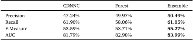
improvement) while the AUC reached 83.99% (a 1.01% improvement).
Moreover, the corresponding ROC curves provide a subtle (yet useful) visual support for this theory. As we can see inFig. 1, CDNNC and Forest learned differently, hence the differences in their curves. CDNNC slightly outperforms Forest at lower false positive rates, but the relationship is reversed at higher rates. Combining their judgments leads to the dotted Ensemble curve, which outperforms both.
This leads us to believe that deep neural networks might already be useful for bug prediction–even if not by themselves but as parts of a higher level ensemble model.
4.4. The effect of data quantity
Another auxiliary experiment we tried was based on the assumption that“deep learning performs best with large datasets”. And by“large”, we mean data points in at least the millions. While our dataset cannot be considered small by any measure,–it is the most comprehensive unified bug dataset we are aware of–it is still not on the“large dataset”scale.
The question then became the following: how could we empirically show that deep learning would perform better on more data without actually having more data? The answer we came up with inverts the problem: we theorize that if data quantity is proportional to the“domi- nance”of a deep learning strategy then it would also manifest as a faster deterioration than the other algorithms when even less data is available.
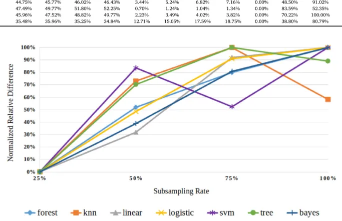
So we artificially shrank–i.e., did a uniform stratified downsampling on –the full dataset three times to produce a 25%, a 50%, and a 75% subset to replicate our whole previous process on. The results are summarized in Table 15.
The table consists of three regions, namely the various F-measures evaluated on their test sets (left), the difference between the best deep learning strategy and the current algorithm (middle), and the same dif- ference, only normalized into the [0,1] interval (right). The normalized relative differences are also illustrated inFig. 2, where the slope of the lines represent the change in the respective differences. So we track these relative differences over changing dataset sizes, and the steeper the incline of the lines, thelessinfluence dataset sizes have over their cor- responding algorithms compared to neural networks.
An imaginaryy¼xdiagonal line would mean that deep learning is linearly more sensitive to more data, which would lead us to believe that if there were any more data, we could linearly increase our performance.
And what we see inFig. 2is not far off from this theoretical indicator. In the case of logistic vs. cdnnc, for example, growth in the differences means that cdnnc is leaving logistic farther and farther behind as more data becomes available. While in the case of forest vs. cdnnc, it means that cdnnc is“catching up” –since thefigures are negative, but their absolute values are decreasing.
As most tendencies of the changing differences empirically corrobo- rate, more data is good for every algorithm, but it has a bigger impact on deep learning. Naturally, there are occasional swings like SVM’s decrease at 75%–possibly due to the more“hectic”nature of the technique–or KNN’s“hanging tail”at 100%. If we assume a linear kind of relationship, however, even these cases show overall growth. This leads us to speculate that deep neural networks could dominate their opponents–individu- ally, even without resorting to the previously described model combi- nation–when used in conjunction with larger datasets. We also note that scalability should not be an issue, as larger input datasets would affect only thetrainingtimes of the models–which is usually an acceptable up- front sacrifice–while leaving prediction speeds unchanged.
5. Threats to validity
Throughout this study, we aimed to remain as objective as possible by disclosing all our presuppositions and publishing only concrete, repli- cable results. However, there are still factors that could have skewed the conclusions we drew. One is the reliability of the bug dataset we used as our input. Building on faulty data will lead to faulty results–also known as the“garbage in, garbage out”principle–but we are confident that this is not the case here. The dataset is independently peer reviewed, accepted, and is compiled using standard data mining techniques.
Another factor might be–ironically–bugs in our bug prediction framework. We tried to combat this by rigorous manual inspections, tests, and replications. Additionally, we are also making the source code openly available on GitHub and invite community verification or comments.
Yet another factor could be the study dimensions we decided tofix– namely, the preprocessing technique, the preliminary resamplig, the number of consecutive misses before stopping early, the 0.5 multiplier for the learning rate“halving”, and even the random seed, which was the same for every execution. Analyzing how changes to these parameters would impact the results–if at all–was out of the scope of this study.
Finally, the connections and implications we discovered from the objectivefigures might just be coincidences. Although there are perfectly logical and reasonable explanations for the unveiled behavior–which we discussed–there is still much to be examined and confirmed in this domain.
Table 12
Forest confusion matrix.
Predicted
Bugged Not Bugged
Measured Bugged 5098 3682
Not Bugged 5105 33,733
Table 13
Ensemble confusion matrix.
Predicted
Bugged Not Bugged
Measured Bugged 5360 3420
Not Bugged 5255 33,583
Table 14
Comparison of individual and ensemble results.
CDNNC Forest Ensemble
Precision 47.24% 49.97% 50.49%
Recall 61.90% 58.06% 61.05%
F-Measure 53.59% 53.71% 55.27%
AUC 81.79% 82.98% 83.99%
Fig. 1.ROC comparison for CDNNC, Forest, and their Ensemble.
6. Conclusions and future work
In this paper, we presented a detailed approach on how to apply deep neural networks to predict the presence of bugs in classes from static source code metrics alone. While neither deep learning nor bug predic- tion are new topics in themselves, we aim to benefit their intersection by combining ideas and best practices from both.
Our greatest contribution is the thorough, step by step description of our process which–apart from the underexplored coupling of concepts– leads to a deep neural network that is on par with random forests and dominates everything else. Additionally, we unveiled that an ensemble model made from our best deep neural network and forest classifiers is actually better than either of its components individually,–suggesting that deep learning is applicable right now–and that more data is likely to make our approach even better. These are two further convincing argu- ments supporting the assumption that the increased time and resource requirements of training a deep learning model are worth it. Moreover, we open-sourced the experimental tool we used to reach these conclu- sions and invite the community to build on ourfindings.
Our future plans include comparing the effectiveness of static source code metrics to change-based and vector embedding-based features when utilized with the same deep learning techniques, and to quantify the effects of different network architectures. We would also like to replicate the outlined experiments with extra tweaks to the parameters we consideredfixed thus far (e.g., the random seed or the preprocessing methodology), thereby examining how stable and resistant to noise our
results are. Additionally, we plan to expand the dataset–ideally some- what automatically to be able to reach an official“large dataset”status in the near future–and to integrate the current best bug prediction model into the OpenStaticAnalyzer toolchain to issue possible bug warnings alongside the existing source code metrics. In the meantime, we consider ourfindings a successful step towards understanding the role deep neural networks can play in bug prediction.
Acknowledgment
This work was partially supported by grant 2018–1.2.1-NKP-2018- 00004“Security Enhancing Technologies for the IoT” funded by the Hungarian National Research, Development and Innovation Office.
Ministry for Innovation and Technology, Hungary grant TUDFO/
47138–1/2019-ITM is acknowledged. The Titan Xp used for this research was donated by the NVIDIA Corporation.
References
[1] Zhivich M, Cunningham RK. The real cost of software errors. IEEE Secur. Priv. 2009;
7(2):87–90.
[2] Ferenc R, Toth Z, Ladanyi G, Siket I, Gyimothy T. A public unified bug dataset for java. In: Proceedings of the 14th international conference on predictive models and data analytics in software engineering. New York, NY, USA: PROMISE’18, ACM;
2018. p. 12–21.https://doi.org/10.1145/3273934.3273936. URL http://
doi.acm.org/10.1145/3273934.3273936.
Table 15
F-measures across different data quantities.
Algorithm Test results Relative difference Normalized relative difference
25 50 75 100 25 50 75 100 25 50 75 100
sdnnc 47.66% 50.73% 51.27% 53.37%
cdnnc 48.19% 51.01% 52.84% 53.59%
forest 50.02% 51.96% 53.31% 53.71% 1.83% 0.95% 0.47% 0.12% 0.00% 51.88% 79.92% 100.00%
knn 48.09% 49.55% 50.88% 52.40% 0.10% 1.46% 1.96% 1.19% 0.00% 73.04% 100.00% 58.27%
linear 43.91% 45.55% 45.16% 45.61% 4.28% 5.46% 7.68% 7.98% 0.00% 31.81% 91.93% 100.00%
logistic 44.75% 45.77% 46.02% 46.43% 3.44% 5.24% 6.82% 7.16% 0.00% 48.50% 91.02% 100.00%
svm 47.49% 49.77% 51.80% 52.25% 0.70% 1.24% 1.04% 1.34% 0.00% 83.59% 52.35% 100.00%
tree 45.96% 47.52% 48.82% 49.77% 2.23% 3.49% 4.02% 3.82% 0.00% 70.22% 100.00% 89.02%
bayes 35.48% 35.96% 35.25% 34.84% 12.71% 15.05% 17.59% 18.75% 0.00% 38.80% 80.79% 100.00%
Fig. 2. The tendencies of the normalized relative differences.
[3] Glorot X, Bordes A, Bengio Y. Deep sparse rectifier neural networks. In: Proceedings of the fourteenth international conference on artificial intelligence and statistics;
2011. p. 315–23.
[4] El Emam K, Melo W, Machado JC. The prediction of faulty classes using object- oriented design metrics. J Syst Software 2001;56(1):63–75.
[5] Subramanyam R, Krishnan MS. Empirical analysis of ck metrics for object-oriented design complexity: implications for software defects. IEEE Trans Software Eng 2003;29(4):297–310.
[6] Gyimothy T, Ferenc R, Siket I. Empirical validation of object-oriented metrics on open source software for fault prediction. IEEE Trans Software Eng 2005;31(10):
897–910.
[7] Nagappan N, Ball T. Static analysis tools as early indicators of pre-release defect density. In: Proceedings of the 27th international conference on Software engineering. ACM; 2005. p. 580–6.
[8] Nagappan N, Ball T, Zeller A. Mining metrics to predict component failures. In:
Proceedings of the 28th international conference on Software engineering. ACM;
2006. p. 452–61.
[9] Nagappan N, Ball T. Use of relative code churn measures to predict system defect density. In: Proceedings of the 27th international conference on Software engineering. ACM; 2005. p. 284–92.
[10] Hassan AE. Predicting faults using the complexity of code changes. In: Proceedings of the 31st international conference on software engineering. IEEE Computer Society; 2009. p. 78–88.
[11] Moser R, Pedrycz W, Succi G. A comparative analysis of the efficiency of change metrics and static code attributes for defect prediction. In: Proceedings of the 30th international conference on Software engineering. ACM; 2008. p. 181–90.
[12] Bernstein A, Ekanayake J, Pinzger M. Improving defect prediction using temporal features and non linear models. In: Ninth international workshop on Principles of software evolution: in conjunction with the 6th ESEC/FSE joint meeting. ACM;
2007. p. 11–8.
[13] Kamei Y, Shihab E, Adams B, Hassan AE, Mockus A, Sinha A, Ubayashi N. A large- scale empirical study of just-in-time quality assurance. IEEE Trans Software Eng 2013;39(6):757–73.
[14] Menzies T, Milton Z, Turhan B, Cukic B, Jiang Y, Bener A. Defect prediction from static code features: current results, limitations, new approaches. Autom Software Eng 2010;17(4):375–407.
[15] D’Ambros M, Lanza M, Robbes R. An extensive comparison of bug prediction approaches. In: Mining software repositories (MSR), 2010 7th IEEE working conference on. IEEE; 2010. p. 31–41.
[16] Shuai B, Li H, Li M, Zhang Q, Tang C. Software defect prediction using dynamic support vector machine. In: Computational intelligence and security (CIS), 2013 9th international conference on. IEEE; 2013. p. 260–3.
[17] Wang J, Shen B, Chen Y. Compressed c4. 5 models for software defect prediction.
In: Quality software (QSIC), 2012 12th international conference on. IEEE; 2012.
p. 13–6.
[18] Ghotra B, McIntosh S, Hassan AE. Revisiting the impact of classification techniques on the performance of defect prediction models. In: Proceedings of the 37th international conference on software engineering, vol. 1. IEEE Press; 2015.
p. 789–800.
[19] Rajbahadur GK, Wang S, Kamei Y, Hassan AE. The impact of using regression models to build defect classifiers. In: Proceedings of the 14th international conference on mining software repositories. IEEE Press; 2017. p. 135–45.
[20] Hinton GE, Salakhutdinov RR. Reducing the dimensionality of data with neural networks. Science 2006;313(5786):504–7.
[21] D. Cires¸an, U. Meier, J. Schmidhuber, Multi-column deep neural networks for image classification, arXiv preprint arXiv:1202.2745.
[22] Krizhevsky A, Sutskever I, Hinton GE. Imagenet classification with deep convolutional neural networks. In: Advances in neural information processing systems; 2012. p. 1097–105.
[23] Toth L. Phone recognition with deep sparse rectifier neural networks. In: Acoustics, speech and signal processing (ICASSP), 2013 IEEE international conference on.
IEEE; 2013. p. 6985–9.
[24] Mohamed A-r, Dahl GE, Hinton G, et al. Acoustic modeling using deep belief networks. IEEE Trans. Audio Speech Lang. Process 2012;20(1):14–22.
[25] Mnih A, Hinton GE. A scalable hierarchical distributed language model. In:
Advances in neural information processing systems; 2009. p. 1081–8.
[26] Sarikaya R, Hinton GE, Deoras A. Application of deep belief networks for natural language understanding. IEEE/ACM Trans. Audio Speech Lang. Process.(TASLP) 2014;22(4):778–84.
[27] Yang X, Lo D, Xia X, Zhang Y, Sun J. Deep learning for just-in-time defect prediction. QRS; 2015. p. 17–26.
[28] Wang S, Liu T, Tan L. Automatically learning semantic features for defect prediction. In: Software engineering (ICSE), 2016 IEEE/ACM 38th international conference on. IEEE; 2016. p. 297–308.
[29] M. Pradel, K. Sen, reportDeep learning tofind bugs, [Technical Report].
[30] Lam AN, Nguyen AT, Nguyen HA, Nguyen TN. Combining deep learning with information retrieval to localize buggyfiles for bug reports (n). In: Automated software engineering (ASE), 2015 30th IEEE/ACM international conference on, IEEE; 2015. p. 476–81.
[31] Lam AN, Nguyen AT, Nguyen HA, Nguyen TN. Bug localization with combination of deep learning and information retrieval. In: Program comprehension (ICPC). IEEE:
IEEE/ACM 25th International Conference on; 2017. p. 218–29. 2017.
[32] Huo X, Li M, Zhou Z-H. Learning unified features from natural and programming languages for locating buggy source code. IJCAI; 2016. p. 1606–12.
[33] Manjula C, Florence L. Deep neural network based hybrid approach for software defect prediction using software metrics. Cluster Comput 2019;22(4):9847–63.
[34] Pascarella L, Palomba F, Bacchelli A. Re-evaluating method-level bug prediction. In:
2018 IEEE 25th international conference on software analysis, evolution and reengineering (SANER). IEEE; 2018. p. 592–601.
[35] Clemente CJ, Jaafar F, Malik Y. Is predicting software security bugs using deep learning better than the traditional machine learning algorithms?. In: 2018 IEEE international conference on software quality, reliability and security (QRS). IEEE;
2018. p. 95–102.
[36] Giger E, D’Ambros M, Pinzger M, Gall HC. Method-level bug prediction. In:
Proceedings of the ACM-IEEE international symposium on Empirical software engineering and measurement. ACM; 2012. p. 171–80.
[37] Jayanthi R, Florence L. Software defect prediction techniques using metrics based on neural network classifier. Cluster Comput 2019;22(1):77–88.
[38] Li J, He P, Zhu J, Lyu MR. Software defect prediction via convolutional neural network. In: 2017 IEEE international conference on software quality, reliability and security (QRS). IEEE; 2017. p. 318–28.
[39] Capretz LF, Xu J. An empirical validation of object-oriented design metrics for fault prediction. J Comput Sci 2008;4(7):571.
[40] ArarOF, Ayan K. Software defect prediction using cost-sensitive neural network.€ Appl Soft Comput 2015;33:263–77.
[41] Gyimothy T, Ferenc R, Siket I. Empirical validation of object-oriented metrics on open source software for fault prediction. IEEE Trans Software Eng 2005;31(10):
897–910.
[42] Gupta DL, Saxena K. Software bug prediction using object-oriented metrics.
Sadhana 2017;42(5):655–69.
[43] Menzies T, Krishna R, Pryor D. The promise repository of empirical software engineering data. 2015.http://openscience.us/repo.
[44] D’Ambros M, Lanza M, Robbes R. An extensive comparison of bug prediction approaches. In: 7th working conference on mining software repositories (MSR).
IEEE; 2010. p. 31–41.
[45] Toth Z, Gyimesi P, Ferenc R. A public bug database of github projects and its application in bug prediction. In: International conference on computational science and its applications. Springer; 2016. p. 625–38.
[46] OpenStaticAnalyzer static code analyzer. 2018.https://github.com/sed-inf-u-s zeged/OpenStaticAnalyzer.
[47] Abadi M, Agarwal A, Barham P, Brevdo E, Chen Z, Citro C, Corrado GS, Davis A, Dean J, Devin M, Ghemawat S, Goodfellow I, Harp A, Irving G, Isard M, Jia Y, Jozefowicz R, Kaiser L, Kudlur M, Levenberg J, Mane D, Monga R, Moore S, Murray D, Olah C, Schuster M, Shlens J, Steiner B, Sutskever I, Talwar K, Tucker P, Vanhoucke V, Vasudevan V, Viegas F, Vinyals O, Warden P, Wattenberg M, Wicke M, Yu Y, Zheng X. TensorFlow: large-scale machine learning on heterogeneous systems. software available from: tensorflow.org. 2015. URL,htt p://tensorflow.org/.
[48] Pedregosa F, Varoquaux G, Gramfort A, Michel V, Thirion B, Grisel O, Blondel M, Prettenhofer P, Weiss R, Dubourg V, Vanderplas J, Passos A, Cournapeau D, Brucher M, Perrot M, Duchesnay E. Scikit-learn: machine learning in Python.
J Mach Learn Res 2011;12:2825–30.
[49] DeepBugHunter–experimental python framework for deep learning. 2019.https ://github.com/sed-inf-u-szeged/DeepBugHunter.
[50] Johnson D. Quicknet. 2019. URL,http://www1.icsi.berkeley.edu/Speech/qn.html.
[51] Goodfellow I, Bengio Y, Courville A. Deep learning. MIT Press; 2016.http://www.d eeplearningbook.org.
[52] Opitz D, Maclin R. Popular ensemble methods: an empirical study. J Artif Intell Res 1999;11:169–98.