Power spectrum estimation of spherical random fields based on covariances ∗
Ágnes Baran, György Terdik
Faculty of Informatics, University of Debrecen baran.agnes@inf.unideb.hu
terdik.gyorgy@inf.unideb.hu
Submitted September 15, 2014 — Accepted November 20, 2014
Abstract
A Gaussian isotropic stochastic field on a 2D-sphere is characterized by either its covariance function or its angular spectrum. The object of this paper is the estimation of the spectrum in two steps. First we estimate the covariance function, secondly we approximate the series expansion of the covariance function with respect of Legendre polynomials. Simulations show that this method is fast and precise.
Keywords:Angular correlation, angular spectrum, isotropic fields on sphere, estimation of correlation
MSC:60G60, 62M30
1. Introduction
There are several physical phenomena which can be described with the help of a spherical random processes. A typical example of random data measured on the surface of a sphere is the cosmic microwave background radiation (CMB). Similar random fields arise in medical imaging, in analysis of gravitational and geomagnetic data etc.. These fields are characterized by a series expansion with respect to the spherical harmonics. Under assumption of Gaussianity both the covariance function and the angular power spectrum describe completely the probability structure of
∗The publication was supported by the TÁMOP-4.2.2.C-11/1/KONV-2012-0001 project. The project has been supported by the European Union, co-financed by the European Social Fund.
http://ami.ektf.hu
15
an isotropic stochastic field. The estimated spectrum can be used to check the underlying physical theory, while the possible non-Gaussianity can be investigated by estimating the higher order angular spectra.
1.1. Notations
LetS2denote the surface of the unit sphere inR3, andX(L)be a random field on S2, where the locationL= (ϑ, ϕ), andϑ∈[0, π]is the co-latitude, whileϕ∈[0,2π]
is the longitude. If the spatial processX(L)is mean square continuous, then it has a series expansion in terms of spherical harmonics Y`m. Spherical harmonics are defied by the Legendre polynomials
P`(x) = 1 2``!
d`
dx`(x2−1)`, x∈[−1,1], (`= 0,1,2, . . .) and the associated Legendre functions
P`m= (−1)m(1−x2)m/2 dm dxmP`(x),
of degree ` and order m, where ` = 0,1,2, . . ., and m = −`, . . . , `. Now the complex valued spherical harmonics of degree ` and orderm (` = 0,1,2, . . ., and m=−`, . . . , `) are given by
Y`m(ϑ, ϕ) =λm` (cosϑ)eimϕ, where
λm` (x) =
s2`+ 1 4π
(`−m)!
(`+m)!P`m(x), ifm≥0, and
λm` (x) = (−1)mλ|m|` (x), ifm <0, that implies
Y`−m(ϑ, ϕ) = (−1)mY`m(ϑ, ϕ).
Using these notations the spherical harmonics expansion of the random field X(L)∈L2(S2)is
X(L) = X∞
`=0
X`
m=−`
Z`mY`m(L),
where the coefficients
Z`m, `= 0,1, . . . , m=−`, . . . , `
are complex valued centered random variables, while puttingEZ00=µimplies that EX(L) =µand the coefficients are given by
Z`m= Z
S2
X(L)Y`m(L)dL, (1.1)
and
Z`m= (−1)mZ`−m.
2. Spectrum
Definition. The random fieldX(L)is called strongly isotropic if all finite dimen- sional distributions of{X(L), L∈S2} are invariant under the rotationg for every g∈SO(3), whereSO(3)denotes the special orthogonal group of rotations defined onS2.
If the spatial processX is strongly isotropic, then E(Z`m11Z`m22) =f`1δ`1`2δm1m2
for `1, `2 ∈N, and mi =−`i, . . . , `i, whereδ`k = 1 if ` = k and zero otherwise, while
E(Z00Z`m) = f0+E(Z00)2
δ0`δ0m, f0=V ar Z00 .
f` =V ar(Z`m), `= 0,1,2, . . ., are nonnegative real numbers, and (f`, `∈ N0) is called the angular power spectrum of the random fieldX. Note E(X) =µ, hence C2(L1, L2) =E(X(L1)−µ)(X(L2)−µ)is the covariance function of the isotropic field X(L). Due to the isotropy the covarianceC2(L1, L2)depends on the angular distanceγ of the locationsL1 andL2 only (wherecosγ=L1·L2). That means
C2(L1, L2) =C2(gL2L1L1, N) =:C(cosγ),
where gL2L1 is the rotation which takesL2into the north pole N andL1into the planexOz.
It is straightforward (see [5]) that C(cosγ) =
X∞ 0
f`
2`+ 1
4π P`(cosγ). (2.1)
For the practical computation of the spectrumfkthe orthogonality of the Legendre polynomials can be used: witht= cos(γ)from (2.1) follows
Z1
−1
C(t)P`(t)dt=f`2`+ 1 4π
Z1
−1
[P`(t)]2dt=f`· 1 2π,
that is
f`= 2π Z1
−1
C(t)P`(t)dt, (2.2)
for`= 0,1,2, . . ..
Example (Lapalce-Beltrami model on S2). Consider the homogeneous isotropic field X onR3according to the equation
4 −c2
X =∂W, where 4 = ∂x∂22
1 +∂x∂22 2 +∂x∂22
3, denotes the Laplace operator on R3. Its spectrum, see ([6]), is
S(λ) = 2 (2π)2
λ2
(λ2+c2)2, λ2=k(λ1, λ2, λ3)k2, with covariance of Matérn Class
C(r) = 1 (2π)3/2
(cr)1/2K1/2(cr)
2c ,
whereK1/2 is the modified Bessel (Hankel) function, see [1].
Now according to the Lapalce-Beltrami operator, which is the restriction of4onto the unit sphereS2,
4B = 1 sinϑ
∂
∂ϑ
sinϑ ∂
∂ϑ
+ 1
sin2ϑ
∂2
∂ϕ2, we consider the stochastic model
4B−c2
XB =∂WB,
on sphere. The covariance function C0 of XB is the restriction of the covariance functionC ofX on sphere andC0(cosγ) =C(2 sin (γ/2)), i.e.
C0(cosγ) = 1 (2π)3/2
rsin (γ/2)
2c K1/2(2csin (γ/2)).
We apply the Poisson formula whenΦ (dλ) =S(λ)dλ, and we obtain the spectrum forXB
f`= 2π2 Z∞
0
J`+1/22 (λ)1 λ
2 (2π)2
λ2 (λ2+c2)2dλ
= Z∞
0
J`+1/22 (λ) λ
(λ2+c2)2dλ.
3. HEALPix
The most widely used pixelisation of the sphere for sampling and analyzing CMB data is the HEALPix (Hierarchical, Equal Area and isoLatitude Pixelization), see
[2]. Actually the CMB data are given on the surface of a unit ball at the discrete points defined by HEALPix. Here in the base resolution partitioning the surface of the sphere is divided into12quadrilateral pixels of same area, and in each further resolution the pixels are subdivided into 4 equal area pixels. Denoting by Nside
the resolution parameter, the total number of pixels equals12Nside2 , and the pixel centers are located on4Nside−1isolatitude rings. Unfortunately, the pixelisation is not rotational invariant, the pixel centers can be rotated into each other in the case of some rotations around the north-south axes only.
4. Computational results
Let us suppose that we are given an observation of an isotropic field on the sphere, more precisely for each HEALPix pixelLwe have a valueX(L). The estimator of the spectrum of the field can be based either on (1.1) or on (2.1). It means that we can approximate the integral (1.1), then for each fixed` we estimatef` as the variance of approximatedZ`m,m=−`, . . . , `. In this case one can not expect good result for small `, since the estimator of the variance f` based on 2`+ 1 values.
The alternative method is based on the estimation of covariance function first then use the expansion (2.1) according to the Legendre polynomials for estimatingf`. The advantage of this later one is that there are many distances between pixels in which the estimation of the covariance is possible.
For further improvement of this computations we are going to apply some sam- pling theorems concerning on spherical harmonics and Legendre polynomials. We show this method through simulations.
In our simulations we consider random fields not only with zero mean but with f0 = 0 as well. The reason is that we have only one realization and when we center the observation the sample mean contains a value ofZ00hencef0can not be identified.
To the numerical approximation of the integral (2.2) denote byt1, t2, . . . , tn the nodes of the quadrature (−1≤ti≤1), and for a givenilet(Li1j, Li2j),j= 1, . . . , N, be pairs of pixels which have angular distanceti. Considering the samples
X1, X2, . . . , XN, where Xj =X(Li1j), and
Y1, Y2, . . . , YN, where Yj=X(Li2j), we use the empirical covariance
Cbi= 1 N
XN
j=1
XjYj
to estimate the valueC(ti),i= 1, . . . , n.
In the program we used only pixels located in the equatorial area (i.e. pixel centers with co-latitude −13 ≤ cosϑ ≤ 13). E.g. in the case of Nside = 16these
pixels determine nearly 9000 different values for t. In the equatorial zone each ring contains the same number of pixels (4Nside), moreover the pixel centers are equidistant located. In order to calculate the possible values of t = cosγ we considered the first pixel center on each ring in the north equatorial belt together with the pixel centers located on and below the actual ring. More precisely it is suffices to consider on each ring only the half of the pixels. After that for a given t to collect the pixel-pairs having distance t we can use the rotation symmetry.
Depending on the location of the original pixel-pair (L1, L2), which was used to compute t, there exist4Nside, 8Nside or 16Nside pairs having the given distance.
If both of the pixels lie on the equator, or θ1 = π−θ2 and ϕ1 = ϕ2 (where L1 = (θ1, ϕ1),L2= (θ2, ϕ2)), that is the locations are symmetric to the equator, then the number of pairs is equal to4Nside. In the case ofθ1=θ26=π2 and in the case of θ16=π−θ2 and ϕ1 =ϕ2, moreover ifθ1 =π−θ2 andϕ1 6=ϕ2, there are 8Nsidepairs. In all other cases there exist16Nsidepairs corresponding to the given distance.
By the numerical calculation of (2.2) using the Gaussian quadrature instead of the built-in Matlab functiontrapz enables a more efficient calculation, since these method requires much less evaluations of empirical covariances, however, this could be subject of further investigations.
Test example 1. (See Figure 1.) As a first example we considered the spatial process
X(L) = X100
`=1
pf`
X`
m=−`
Z`mY`m(L), (4.1)
whereZ`m∼ N(0,2) are i.i.d. random numbers and
f`= 1
(`(`+ 1) + 4)2, `= 1,2, . . .
−0.2 −0.15 −0.1 −0.05 0 0.05 0.1 0.15 0.2 0.25 0.3
Figure 1: A random field described in Test example 1
By the discretization of the sphere we usedNside= 16as resolution parameter, which results 3072 pixels located on 63 isolatitude rings.
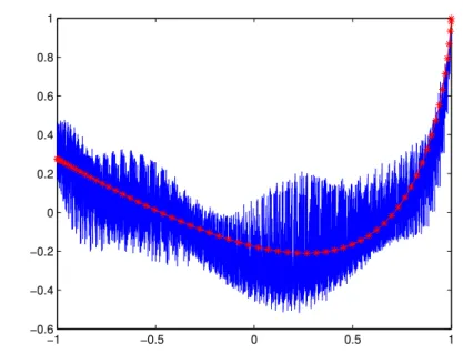
The estimated and theoretical correlations can be seen on Figure 2 such that f0=f1= 0.
−1 −0.5 0 0.5 1
−0.6
−0.4
−0.2 0 0.2 0.4 0.6 0.8 1
Figure 2: Estimated correlation in Test example 1
Let us denote byfˆ`,`= 1, . . . ,100the estimated spectrum, then we obtained X100
`=1
(f`−fˆ`)2≈1.93·10−4
and
1≤max`≤100|f`−fˆ`|= 4.2·10−3.
Test example 2. In the second example we investigated the field defined by the sum (4.1) taking
f`= 4π
2`+ 10.8`, `= 1,2, . . .
The covariance is estimated from the generated field, and the theoretical correlation
C(γ) = 1
p1−1.6 cosγ+ 0.82 −1;
are shown on Figure 3.
−1 −0.5 0 0.5 1
−0.8
−0.6
−0.4
−0.2 0 0.2 0.4 0.6 0.8 1
Figure 3: Estimated correlation in Test example 2
References
[1] Abramowitz, M., Stegun, I.A.,Handbook of mathematical functions with formu- las, graphs and mathematical tables,Dover Publications Inc., New York, (1992) [2] Górski, K.M., Hivon, E., Banday, A. J., Wandelt, B.D., Hansen, F.K.,
Reinecke, M., Bartelmann, M., HEALPix: A framework for high-resolution dis- cretization and fast analysis of data distributed on the sphere, The Astrophysical Journal, Vol. 622 (2005), 759–771.
[3] Lang, A., Schwab, C.,Isotropic Gaussian Random Fields on the Sphere, Regularity, Fast Simulation, and Stochastic Partial differential Equations,arXiv:1305.1170v1 [4] Marinucci, D., Peccati, G.,Random fields on the Sphere, Cambridge University
Press, Cambridge, (2011)
[5] Terdik, Gy.,Angular Spectra for non-Gaussian Isotropic Fields,arXiv:1302.4049v2, to appear Brazilian Journal of Probability and Statistics,http://imstat.org/bjps/
papers/BJPS249.pdf
[6] Yadrenko, M. I.,Spectral theory of random fields,Optimization Software Inc. Pub- lications Division, New York, (1983)