Using GPUs to accelerate computational diffusion MRI: From microstructure estimation to tractography and connectomes
Moises Hernandez-Fernandez
a,b,*, Istvan Reguly
c, Saad Jbabdi
a, Mike Giles
d, Stephen Smith
a, Stamatios N. Sotiropoulos
a,eaWellcome Centre for Integrative Neuroimaging - Centre for Functional Magnetic Resonance Imaging of the Brain (FMRIB), University of Oxford, Oxford, United Kingdom
bCenter for Biomedical Image Computing and Analytics (CBICA), Department of Radiology, University of Pennsylvania, Philadelphia, PA, United States
cFaculty of Information Technology and Bionics, Pazmany Peter Catholic University, Budapest, Hungary
dMathematical Institute, University of Oxford, Oxford, United Kingdom
eSir Peter Mansfield Imaging Centre, School of Medicine, University of Nottingham, Nottingham, United Kingdom
A R T I C L E I N F O Keywords:
GPGPU
Scientific computing Biophysical modelling Non-linear optimisation Bayesian inference Fibre orientations Fibre dispersion Brain connectivity Medical imaging
A B S T R A C T
The great potential of computational diffusion MRI (dMRI) relies on indirect inference of tissue microstructure and brain connections, since modelling and tractography frameworks map diffusion measurements to neuroan- atomical features. This mapping however can be computationally highly expensive, particularly given the trend of increasing dataset sizes and the complexity in biophysical modelling. Limitations on computing resources can restrict data exploration and methodology development. A step forward is to take advantage of the computational power offered by recent parallel computing architectures, especially Graphics Processing Units (GPUs). GPUs are massive parallel processors that offer trillions offloating point operations per second, and have made possible the solution of computationally-intensive scientific problems that were intractable before. However, they are not inherently suited for all problems. Here, we present two different frameworks for accelerating dMRI computations using GPUs that cover the most typical dMRI applications: a framework for performing biophysical modelling and microstructure estimation, and a second framework for performing tractography and long-range connectivity estimation. The former provides a front-end and automatically generates a GPU executablefile from a user- specified biophysical model, allowing accelerated non-linear modelfitting in both deterministic and stochastic ways (Bayesian inference). The latter performs probabilistic tractography, can generate whole-brain connectomes and supports new functionality for imposing anatomical constraints, such as inherent consideration of surface meshes (GIFTIfiles) along with volumetric images. We validate the frameworks against well-established CPU- based implementations and we show that despite the very different challenges for parallelising these problems, a single GPU achieves better performance than 200 CPU cores thanks to our parallel designs.
1. Introduction
General-purpose computing on graphics processing units (GPGPU) has lead to a significant step forward in scientific computations. GPUs are massive parallel processors with thousands of cores. Mainly driven by the computer game industry, and more recently by deep learning applica- tions (Schmidhuber, 2015), GPUs have evolved rapidly in the last decade, offering now over 15 TeraFLOPS (151013floating operations per second) in single precision of performance (NVIDIA, 2017). Even if their full potential is not used, their suitability for scientific computing has become more and more evident in projects that involve large
amounts of data. For instance, the 1000 Genomes Project (Auton et al., 2015;Sudmant et al., 2015) and the Human Connectome Project (Van Essen and Ugurbil, 2012;Van Essen et al., 2012;Sotiropoulos et al., 2013) have generated Petabytes of data. The computations performed for the analysis of all this data can take months on typical computer clusters, but GPU accelerated solutions can accelerate massively these computa- tions (Klus et al., 2012;Hernandez et al., 2013).
In thefield of medical imaging, GPUs have been used in several computational domains (Eklund et al., 2013), including image recon- struction (Stone et al., 2008;Uecker et al., 2015) image segmentation (Smistad et al., 2015; Alsmirat et al., 2017), image registration
* Corresponding author. Wellcome Centre for Integrative Neuroimaging - Centre for Functional Magnetic Resonance Imaging of the Brain (FMRIB), University of Oxford, Oxford, United Kingdom.
E-mail address:moisesf@fmrib.ox.ac.uk(M. Hernandez-Fernandez).
Contents lists available atScienceDirect
NeuroImage
journal homepage:www.elsevier.com/locate/neuroimage
https://doi.org/10.1016/j.neuroimage.2018.12.015
Received 28 June 2018; Received in revised form 20 November 2018; Accepted 7 December 2018 Available online 8 December 2018
1053-8119/Crown Copyright©2018 Published by Elsevier Inc. This is an open access article under the CC BY license (http://creativecommons.org/licenses/by/4.0/).
–
(Shamonin, 2014), and in the analysis of functional MRI (Eklund et al., 2014) and diffusion MRI data (Xu et al., 2012;Hernandez et al., 2013;
Chang et al., 2014; Hernandez-Fernandez et al., 2016; Harms et al., 2017).
However, using GPUs is not always straightforward. The GPU archi- tecture is completely different to the traditional single or multi-core CPU architectures, it is not inherently suited for all types of problems, and bespoke computational frameworks may need to be developed to take advantage of their full potential. Some of the challenges that need to be considered for achieving an efficient design include: balanced paralleli- sation of an algorithm, good organisation of threads and grouping, appropriate usage of memory resources, appropriate memory access patterns, and correct communication and synchronisation between threads. Furthermore, programming GPUs requires specific program- ming models that offer control over the device resources, but may in- crease the difficulty for designing parallel solutions. Low-level programming models, such as the Compute Unified Device Architecture (CUDA) (Nickolls et al., 2008), offer a high degree of control over the resources, and the possibility of achieving very efficient solutions. A more detailed description of the GPU architecture, the CUDA program- ming model, and some considerations for GPU programming are included in the Supplementary material.
Despite the challenges, in this paper we illustrate the potential of GPUs for two neuroimaging applications spanning different parallelisa- tion strategies. Specifically, we design and implement parallel compu- tational frameworks for analysing diffusion magnetic resonance imaging (dMRI) data (Alexander et al., 2017;Jeurissen et al., 2017;Sotiropoulos and Zalesky, 2017). The great potential of dMRI is that it uniquely allows studying the human brain non-invasively and in vivo. However, it relies on indirect inference from the data, and typically, modelling frameworks are necessary to map dMRI measurements to neuroanatomical features, which can be computationally expensive. The computational cost is becoming even higher given the trend of increasing data sizes. New MRI hardware and sequences for pushing spatial and angular resolution (Vu et al., 2015;Setsompop et al., 2018) can considerably increase the size of a single subject dataset. At the same time, big imaging data repositories with a large number of subjects are being created, such as the Human Connectome Project (HCP) (Van Essen and Ugurbil, 2012;Van Essen et al., 2012;Sotiropoulos et al., 2013), where 1200 datasets are included, its Lifespan and Disease extensions (https://www.humanconnectome.
org) and UK Biobank (Miller et al., 2016;Alfaro-Almagro et al., 2018) where a total of 100,000 subjects are being scanned. Limitations in computing can restrict data exploration and even methodology development.
A common application of dMRI analysis is tissue microstructure estimation. Even if the diffusion tensor imaging model (DTI) (Basser et al., 1994a,b) is by far the most popular framework for extracting microstructure indices and can befitted linearly to data, it has major limitations such as the inability to capture partial volume, leading to non-specific markers of tissue structural changes (Basser et al., 2000;
Poupon et al., 2000;Wiegell et al., 2000;Alexander et al., 2001;Pierpaoli et al., 2001;Seunarine and Alexander, 2014). To overcome these limi- tations, multi-compartment biophysical models are being developed, where the diffusion signal attenuation is represented as a mixture of signals obtained from different tissue components (Szafer et al., 1995;
Niendorf et al., 1996;Stanisz et al., 1997;Assaf and Cohen, 1998;Mul- kern et al., 1999;Assaf et al., 2008;Alexander et al., 2010;Sotiropoulos et al., 2012;Zhang et al., 2012). Multi-compartment dMRI models are commonly non-linear functions of the signal, and non-linear optimisation algorithms are typically used for fitting the model to the diffusion-weighted measurements (Motulsky and Ransnas, 1987;Kelley, 1999). These algorithms use iterative optimisation procedures forfinding a global solution, leading to potentially large computational times.
Furthermore, if a stochastic (instead of deterministic) optimisation method is required, such as Bayesian approaches (Tarantola, 2005), computation requirements are even heavier. For instance, using a cluster
with 72 CPU cores,fitting the NODDI-Bingham model (Tariq et al., 2016) to a single subject of the UK Biobank dataset with the current available Matlab toolbox (Microstructure Imaging Group - University College London, 2017) requires more than 6 h for deterministicfitting, andfitting the ball and sticks model (Behrens et al., 2003,2007) to a single subject of the HCP dataset with FMRIB's Software Library (FSL) (Jenkinson et al., 2012) requires 5 h for stochasticfitting using MCMC on a large cluster with 145 CPU cores (seeTable 1).
Optimisation methods used forfitting voxel-wise biophysical models to dMRI data are inherently parallelisable and in general well suited for GPU design, since the computational modelling is applied independently to different voxels. The large number of independent elements in the data and the fact that identical procedures need to be performed over each of these elements make GPUs a perfect candidate for processing these datasets, as they have been designed for exploiting the data level paral- lelism by executing the same instructions over different data simulta- neously (SIMD (Flynn, 1972)). However, due to the heavy tasks involved in the optimisation procedures, the design of an optimal parallel solution is non-trivial.
A number of GPU frameworks for accelerating these routines have been developed in the past by ourselves and others focusing on specific models forfibre orientation or diffusion tensor estimation (Xu et al., 2012; Hernandez et al., 2013; Chang et al., 2014). In this paper we reformulate our previous proposed approach (Hernandez et al., 2013) and provide a generic and model independent toolbox for modelfitting using GPUs. The toolbox provides aflexible and friendly front-end for the user to specify a model, define constraints and any prior information on the model parameters, and choose a non-linear optimisation routine, ranging from deterministic Gauss-Newton type approaches to stochastic Bayesian methods based on Markov Chain Monte Carlo (MCMC). It then automatically generates a GPU executablefile that reflects all these op- tions. This achievesflexibility in modelfitting and allows a single GPU to achieve a better performance than 200 CPU cores.
To further explore the potential of GPUs for computational dMRI, we present another parallel framework for white matter tractography and connectome estimation, a common dMRI application with completely different features and challenges compared to the voxel-wise biophysical modelling. We focus here on probabilistic tractography approaches, which for certain applications can be very time consuming (Behrens et al., 2007). For instance, the generation of a“dense” connectome (Sporns et al., 2005) from a single subject using high-resolution data from the HCP can take more than 9 h on a large CPU cluster (seeTable 1). In the case of tractography algorithms, the main challenge for a GPU par- allel solution comes from the fact that the required data for propagating each streamline (set of voxels with distributions offibre orientations) is not known in advance, as their paths are estimated dynamically on the fly. This makes the allocation of GPU resources difficult, and therefore, the a-priori assessment of the parallelisability of the application chal- lenging. Moreover, the streamlines propagation is likely to be asyn- chronous as they may have imbalanced execution length, which induces thread divergence and causes performance degradation on GPUs.
Table 1
Execution times and memory requirements of some dMRI applications processing datasets from the UK Biobank project and the Human Connectome Project.
Processing times are reported using several CPU cores from several modern processors (Intel Xeon E5-2660 v3 processors).
Application (Single subject) Computational resources
Time Memory
Required
Ball&2 sticks model (MCMC) -
UK Biobank
72 cores 0.73 h 2.5 GB
Ball&2 sticks model (MCMC) -
HCP
145 cores 5 h 8 GB
NODDI-Bingham. Multi- compartment model–Biobank
72 cores 6.75 h 2.5 GB
Brain Connectome (dense) - HCP 100 cores 9.5 h 35 GB
Furthermore, these methods have typically high memory requirements and include relatively heavy tasks, particularly for large datasets and whole-brain explorations, making the design of an efficient GPU-accelerated solution (which ideally comprises light and small tasks) even less straightforward. Preliminary GPU parallel tractography frameworks have been proposed in the past (Mittmann et al., 2008;Xu et al., 2012); however, our tractography parallel framework achieves accelerations of more than 200 times compared to CPU-based imple- mentations and includes novel features that allow even more accurate anatomical constraints to be imposed, such as the inherent support of surface meshes (GIFTIfiles (Harwell et al., 2008)), and the possibility of generating dense connectomes.
In summary, we illustrate that, despite differences in parallelisability challenges, well-thought GPU-based designs that are carefully imple- mented can offer the same performance as hundreds of CPU cores, within the different contexts of tissue microstructure estimation, and tractog- raphy and connectome generation. The developed frameworks will be released upon publication within the FSL software library (Jenkinson et al., 2012)1.
2. Material and methods
2.1. Biophysical modelling on GPUs 2.1.1. Framework description
Tissue microstructure estimation from dMRI is typically performed on a voxel-by-voxel basis, where a biophysical model isfitted. Excluding the DTI model, which can be easily and quickly fitted using linear least squares, most models are non-linear and numerical optimisation routines are required. Non-linear optimisation is typically computationally demanding and can be very time consuming, particularly since advanced multi-compartment models (Alexander et al., 2017) require larger than average datasets (multipleb-valuesor high angular resolution).
Given the large number of voxels and the relatively low memory re- quirements of these independent tasks, such an application is well-suited for implementation on GPUs. To take advantage of the inherent paral- lelisability of the problem and yet cover all possible dMRI models, we have developed a generic toolbox for designing and fitting nonlinear models using GPUs and CUDA. The toolbox, CUDA diffusion modelling toolbox (cuDIMOT), offers a friendly andflexible front-end for the users to implement new models without the need for them to write CUDA code or deal with a GPU design, as this is performed by the toolbox auto- matically (Fig. 1). The user only specifies a model using a C-like language header. This model specification includes the model parameters, con- straints and priors for these parameters, the model predicted signal function, and optionally the partial derivatives with respect to each parameter if they can be provided analytically (cuDIMOT offers the op- tion for numerical differentiation). Once the model specification has been provided, the toolbox integrates this information with the parallel CUDA design of the correspondingfitting routines at compilation time, and it generates a GPU executable. Thefitting routines include options for both deterministic (e.g. Gauss-Newton type) and stochastic (e.g.
Bayesian inference using MCMC) optimisation.
An important factor to take into account in the design of the frame- work is its generic and model-independent aspect. In order to achieve an abstraction of the fitting routines, these are implemented in a generic way excluding functions that are model-dependent. The management of threads, definition of grid size and data distribution are also challenging aspects that cuDIMOT automates. Thefitting routines, deterministic and stochastic, are implemented in different CUDA kernels. The toolbox im- plements the different kernels, deals with the arduous task of distributing
the data among thousands of threads, uses the GPU memory spaces efficiently, and even distributes the computation among multiple GPUs if requested. Two levels of parallelism are used in our design (seeFig. 2). A first level distributes thefitting process of all the voxels amongst CUDA warps(groups of 32 CUDA threads). Specifically, thefitting process of a few voxels is assigned to a CUDAblock(a group of CUDA warps), and each warpfits the model to a single voxel. In a second level of paralle- lisation, the computation of the most expensive within-voxel tasks is distributed amongst threads within a warp, including the computation of the model predicted signal and residuals, and the partial derivatives with respect to the model parameters across the different measurement points.
More details about the parallel design and implementation of cuDIMOT are provided in theSupplementary material.
Additionally, a higher-level of parallelism can be further used to enhance even more the performance, using very large groups of voxels and a multi-GPU system. We can divide a single dataset into groups of voxels and assign each group to a different GPU. The different GPUs do not need to communicate because the groups of voxels are completely independent, apart from thefinal step of outputting the results.
In terms of optimisation routines, cuDIMOT offers a number of deterministic and stochastic model-fitting approaches, including greedy optimisation using Grid-Search, non-linear least-squares optimisation using Levenberg-Marquardt (LM) and Bayesian inference using Markov Chain Monte Carlo (MCMC).
MRI models can have free parameters, which are estimated, andfixed parameters, which reflect measurement settings or features that are known. cuDIMOT allows suchfixed parameters to be defined, and these may be common to all voxels or not (CFP or commonfixed parameters and FixP orfixed parameters inSupplementary Fig. 3a). For instance, in typical diffusion MRI, the diffusion-sensitising gradient strengths (b values) and associated directions (b vectors) would be CFPs, whereas for diffusion-weighted steady-state free precession (DW-SSFP) (McNab and Miller, 2008), theflip angle (α) and repetition time (TR) would be CFPs, while the longitudinal and transverse relaxation times (T1 and T2) would be FixP, as they vary across voxels. Using a simple syntax, a list with all the information is passed to the toolbox through the designer interface.
This information is parsed by cuDIMOT and used at execution time, when the model user must provide maps with these parameters. This generic interface allows the users to combine data from dMRI with data from other modalities, such as relaxometry (Deoni, 2010), and develop more complex models (Foxley et al., 2015,2016;Tendler et al., 2018), or, even use cuDIMOT in different modalities where nonlinear optimisation is required.
Prior information or constraints on the parameters of a model can be integrated into thefitting process using the toolbox interfaces, where a simple syntax is used for enumerating the type and the value of the priors (seeSupplementary Fig. 3b). Upper and lower limits or bounds can be defined for any parameter (transformations are implemented internally and described in theSupplementary material), and priors can be any of the following types:
A Normal distribution. The mean and the standard deviation of the distribution must be specified.
A Gamma distribution. The shape and the scale of the distribution must be specified.
Shrinkage prior or Automatic Relevance Determination (ARD) (MacKay, 1995). The factor or weight of this prior must be provided in the specification.
Uniform distribution within an interval and uniform on a sphere (for parameters that describe an orientation).
For stochastic optimisation, a choice can also be made on the noise distribution and type of the likelihood function (Gaussian or Rician).
Because high-dimensional models are difficult tofit without a good initialisation, the toolbox offers an option for cascadedfitting, where a simpler model isfittedfirst, and the estimated parameters are used to
1Current versions of the toolboxes are publicly available on:https://users.
fmrib.ox.ac.uk/~moisesf/cudimot/index.html and https://users.fmrib.ox.ac.
uk/~moisesf/Probtrackx_GPU/index.html.
initialise the parameters of a more complex model. 3D volumes can be used for specifying the initialisation value of the model parameters in every voxel.
Once a model has been defined and an executablefile created, a user still hasflexibility in controlling a number offitting options, including:
Choosing fitting routines: Grid-Search, Levenberg-Marquardt or MCMC. A combination of them is possible, using the output of one to initialize the other.
Selecting number of iterations in Levenberg-Marquardt and MCMC (burn-in, total, sample thinning interval).
Using Gaussian or Rician noise modelling in MCMC.
Choosing model parameters to be kept fixed during the fitting process.
Choosing model selection criteria to be generated, such as BIC and AIC.
2.1.2. Exploring microstructure diffusion MRI models with cuDIMOT We used cuDIMOT for implementing a number of diffusion MRI models and assess the validity of the results. We have implemented the Neurite Orientation Dispersion and Density Imaging (NODDI) model,
using Watson (Zhang et al., 2012) and Bingham (Tariq et al., 2016) distributions for characterising orientation dispersion.
We implemented NODDI-Watson with cuDIMOT using the designer interface. This model assumes the signal comes from three different compartments: isotropic compartment, intra-cellular compartment and extra-cellular compartment. The model has five free parameters: the fraction of the isotropic compartmentfiso, the fraction of the intra-cellular compartment relative to the aggregate fraction of the intra-cellular and extra-cellular compartmentsfintra, the concentration offibre orientations κ(the lower this value the higher the dispersion), and two angles for defining the mean principalfibre orientationθ andϕ. The concentration parameter κ can be transformed and expressed as the orientation dispersion indexODε½0;1:
OD¼2 πarctan
1 κ
(1) We implemented the model predicted signal of NODDI-Watson as in (Zhang et al., 2011), providing analytically the derivatives forfiso,fintra. We used numerical differentiation to evaluate the partial derivatives of the rest of parameters. We used numerical approximations (e.g. for the Dawson's integral) as in (Press et al., 1988), and we performed the same Fig. 1. General design of CUDA Diffusion Modelling Toolbox (cuDIMOT). Two types of users interact with the toolbox through interfaces, a model designer and a model user. The model designer provides the model specification (parameters, priors, constraints, predicted signal and derivatives), whereas the model user interacts with the toolbox forfitting the model to a dataset. The toolbox provides CUDA kernels that implement severalfitting routines. These kernels are combined with the model specification at compilation time for generating a GPU executable application.
Fig. 2. Parallel design of cuDIMOT forfitting dMRI models on a GPU. The V voxels of a dataset are divided into groups of B voxels (voxels per block), and thefitting process of each of these groups is assigned to different CUDA blocks. Inside a block, a warp (32 threads) collaborate for within-voxel computations.
cascaded steps as the Matlab NODDI toolbox (Microstructure Imaging Group - University College London, 2017). First, we fit the diffusion tensor model for obtaining the mean principalfibre orientation (θandϕ).
Second, we run a Grid-Search algorithm testing different combination of values for the parameters fiso, fintra and κ. Third, we run Levenberg-Marquardt algorithmfitting onlyfiso,fintraandfixing the rest of parameters. Finally, we run Levenberg-Marquardt,fitting all the model parameters. The only difference is that the Matlab toolbox uses an active set optimisation algorithm (Gill et al., 1984) instead of Levenberg-Marquardt.
The NODDI-Bingham model assumes the same compartments as NODDI-Watson. However, this model can characterise anisotropic dispersion, and thus it has two concentration parametersκ1,κ2, and an extra angleψwhich is orthogonal to the mean orientation of thefibres, and encodes a rotation of the main dispersion direction. Whenκ1¼κ2
the dispersion is isotropic, and whenκ1>κ2anisotropic dispersion oc- curs. In this case, the orientation dispersion indexODis defined as:
OD¼2 πarctan
ffiffiffiffiffiffiffiffiffiffiffiffiffiffiffiffiffiffiffiffiffiffiffi 1
κ2
1 κ1
s
!
(2)
and an indexDAε½0;1reflecting the factor of anisotropic dispersion can be defined as:
DA¼2 πarctan
κ1κ2
κ2
(3) We implemented NODDI-Bingham using cuDIMOT in a similar manner as the previous model (only providing the analytic derivatives for
thefisoandfintraparameters). For implementing the confluent hypergeo-
metric function 1F1 of a matrix argument, included in the predicted signal of the intra-cellular and extra-cellular compartments of the model, we use the approximation described in (Kume and Wood, 2005). We use the same optimisation steps as in the NODDI-Watson: diffusion tensor fitting, Grid-Search, and Levenberg-Marquardt twice.
2.2. Probabilistic tractography and connectomes on GPUs
Contrary to voxel-wise modelfitting, white-matter tractography, and particularly whole-brain connectome generation, are not inherently suited for GPU parallelisation. Very high memory requirements,uncoal- esced memory accesses and threads divergence (irregular behaviour of threads in terms of accessed memory locations and life duration) are some of the major factors that make a GPU parallel design of such an application challenging. Nevertheless, we present a framework that parallelises the propagation of multiple streamlines for probabilistic tractography and overcomes the aforementioned issues using an over- lapping pipeline-design.
2.2.1. Framework description
We design a parallel design and develop a GPU-based framework for performing probabilistic tractography. Our application includes the common tractography functionality, including for instance options to set:
The number of streamlines propagated from each seed point, i.e., the number of samples.
Streamline termination criteria (maximum number of steps, curva- ture threshold, anisotropy threshold, tract loop detection)
A number of numerical integration approaches, including Euler's method and 2nd order Runge-Kutta method (Basser et al., 2000), with a subsequent choice of step length.
Propagation criteria and anatomical constraint rules (seed, waypoint, termination, stopping, and target masks) (Smith et al., 2012).
Ability to accept tracking protocols in either diffusion or structural/
standard space.
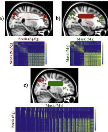
Connectome generation is also inherently supported (Sporns et al., 2005) and three options are available (see Fig. 3) (Li et al., 2012;
Donahue et al., 2016):
Connectivity matrix between all the seed points and all the other seed points. A typical use is for studying the connectivity from all grey matter to all grey matter (Glasser et al., 2013).
Connectivity matrix between all the points of two different masks, which are independent of the seed points mask. A typical use is for studying the connectivity between grey matter regions, when seeding from all white matter.
Connectivity matrix between all the seed points and all the points specified in a different mask. A typical example is to use the whole brain as a target mask for studying the connectivity profile of the grey matter in a specific seed, and use it for connectivity-based classifi- cation (Johansen-Berg et al., 2004).
We have also included an extra feature that is not typically found in tractography toolboxes, but can be important in defining anatomically accurate constraints. We included in our parallel framework the possi- bility of using surfaces, as well as volumes, for defining seed and regions of interest (ROIs). We implement support for the GIFTI format (Harwell et al., 2008), according to which surfaces are defined by meshes of tri- angles. Three spatial coordinates define each triangle vertex in a 3D space. Surface vertices can be used for defining seed points, and mesh triangles can be used for defining stopping/constraint masks. If the latter, a streamline needs to be checked upon crossing the surface meshes. We implement the method described in (O'Rouke, 1998) (ray-plane inter- section) for checking if the segments of a streamline intersects a triangle (details of the method are presented in theSupplementary material).
When designing a parallel solution, we first notice that path
Fig. 3.Connectivity matrices modes offered by the GPU-accelerated tractog- raphy framework. The framework can generate connectivity matrices from a) all seed to all seed points, b) all points in a mask to all points in another mask seeding from an independent region, or c) all seed points to all points in a different mask.
propagation is completely independent across streamlines, and thus it can be in principle parallelised. To reflect that, we can create as many CUDA threads as the required number of streamlines, in fact twice the number of streamlines, as we propagate from each seed point towards both directions indicated by the localfibre orientation. Thus, forDseed points andFstreamlines per seed, we create2DFthreads in total (seeFig. 4). Nevertheless, there are complexities that make such a design challenging and considerably reduce efficiency if not addressed, as we explain below. These include heavy tasks, thread divergence and mem- ory allocation challenges.
Afirst consideration is the high complexity of some of the routines included for implementing the offered functionality. For instance, the use of surfaces involves the execution of an intersection detection algorithm, while the streamline propagation includes interpolation and space transformation routines. Furthermore, checking anatomical constraints during propagation increases the complexity of the algorithm, and in- duces a significant number of conditional branches. Having a single CUDA kernel for performing all these tasks leads to substantially heavy threads, which consume a lot of computational resources and conse- quently cause low occupancy in a GPU Streaming Multiprocessor (SM, seeSupplementary Fig. 1). To solve this issue, we split the application into multiple tasks, each of which is implemented in a different CUDA kernel. A pipelined design is used to execute these kernels, running them serially one after the other. Afirst kernel propagates the streamlines, and subsequently, kernels for checking anatomical constraints, generating path distribution maps and generating connectomes are executed.
Further details of these kernels and the executing pipeline of the appli- cation are included in theSupplementary material.
Another main challenge is related to memory requirements. It may be impossible to use GPUs if the memory demands exceed the available device memory, and typically, this is true across all levels in the GPU memory hierarchy. Tractography algorithms need a distribution offibre orientations for sampling. As we cannot predict the streamline track lo- cations in advance, thefibre orientation distributions of all voxels need to be allocated in memory. The amount of required memory depends on the size (spatial dimensions) of the dataset and for probabilistic tracking on the number of samples in the orientation distributions. For instance, the required memory for simply allocating the samples of a Human Con- nectome Project dataset (Van Essen and Ugurbil, 2012;Van Essen et al., 2012;Sotiropoulos et al., 2013) is approximately 1.5 GB. Moreover, the 3D streamline coordinates need to be stored, but the number of steps that a streamline will take cannot be predicted in advance. We therefore need to allocate enough memory for storing the maximum possible number of coordinates for each streamline. Additionally, volumes and/or surfaces may be used for defining seeds, anatomical constraints and connectome matrix elements, and all of them need also to be allocated in memory.
Our strategy for overcoming this issue was to allocate all the required memory in the GPU without considering the streamline coordinates, and
then propagate the maximum number of streamlines that can be computed in parallel given the amount of memory left. If all the requested streamlines cannot be computed in parallel (which is the most typical scenario), the application iterates over different streamline sets.
Another challenge that limits the performance is thread divergence.
The streamlines may be initialised at different seed points and they can propagate to different regions and for different lengths. This causes ac- cesses to different memory locations when sampling, i.e., uncoalesced memory accesses. Furthermore, streamlines may terminate at different time points. This causes asynchronous thread termination and a possible waste of computational resources, as some threadsfinish their execution before others and stay idle, wasting GPU resources. This situation persists until all the threads of the same CUDA blockfinish their execution and the GPU scheduler switches the block with another block of threads. For this reason, we set the block size K to a small size of 64 threads (2 warps).
Although with this configuration full SM occupancy is not achieved (because there is a limit in the number of blocks per SM), there can be fewer divergences than having larger blocks. Moreover, the GPU can employ the unused resources by overlapping other tasks/kernels in parallel.
We indeed take advantage of our pipelined design and useCUDA streamsto overlap the computation of different sets of streamlines. CUDA streams are queue instances for managing the order of execution of different tasks (NVIDIA, 2015a) and offer the possibility of running concurrently several tasks (kernels execution and/or CPU-GPU memory transfers) on the same GPU. Our framework divides the streamlines into a few sets, and uses a number of OpenMP (Chapman et al., 2008) threads to execute the pipeline of several streamline sets on different CUDA streams concurrently (seeSupplementary Fig. 6b).
2.3. Diffusion–weighted MRI data
The GPU designs presented in this paper have already been used to process hundreds of datasets. Here, we illustrate performance gains on various exemplar data with both high and low spatial resolutions.
For testing the diffusion modelling framework (cuDIMOT) we used data from UK Biobank (Miller et al., 2016). Diffusion-weighting data were acquired using an EPI-based spin-echo pulse sequence in a 3T Siemens Skyra system. A voxel size of 2.02.02.0 mm3 was used (TR¼3.6 s, TE¼92 ms, 32-channel coil, 6/8 partial Fourier) and 72 slices were acquired. Diffusion weighting was applied in M¼100 evenly spaced directions, with 5 directions b¼0 s/mm2, 50 directions b¼1000 s/mm2and 50 directions b¼2000 s/mm2. A multiband factor of 3 was employed (Moeller et al., 2010;Setsompop et al., 2012). A T1 structural image (1 mm isotropic) of the same subject was used for creating a white&grey matter mask, which was non-linearly registered to the space of the diffusion dataset (Andersson et al., 2007), and applied to the map of the estimated parameters before showing the results included in this paper. For creating this mask, a brain extraction tool (Smith, 2002) and a tissue segmentation tool (Zhang et al., 2001) were used.
For testing the GPU probabilistic tractography framework, data were acquired on a 3T Siemens Magnetom Prisma using HCP-style acquisitions (Sotiropoulos et al., 2013). Diffusion-weighting was introduced using single-shot EPI, using an in-plane resolution of 1.351.35 mm2 and 1.35 mm slice thickness (TR¼5.59 s, TE¼94.6 ms, 32-channel coil, 6/8 partial Fourier). 134 slices were acquired in total and diffusion weighting was applied in M¼291 evenly spaced directions, with 21 directions b¼0 s/mm2, 90 directions b¼1000 s/mm2, 90 directions b¼2000 s/mm2and 90 directions b¼3000 s/mm2.
2.4. Hardware features
We used an Intel host system with NVIDIA GPUs and a large cluster of Intel processors for testing our parallel designs. The system has a dual NVIDIA K80 accelerator (Error Correcting Codes ECC enabled), Fig. 4. GPU parallel design of the streamline probabilistic tractography
framework. For each of theDseeds and for each of theFstreamlines per seed, we create two CUDA threads (a and b), which are distributed amongst blocks of K threads.
connected to the host via PCI express v3. A single GPU was used for the experiments. The system has tens of CPU nodes, and each node is comprised of 2 Intel Xeon E5-2660 v3 2.60 GHz processors, each with 10 cores (20 CPU cores per node), and 384 GB (2416 GB) RDIMM mem- ory. Major features of the NVIDIA K80 accelerators and the Intel pro- cessors are summarized in Supplementary Table 1 (NVIDIA, 2014a, 2015b).
The systems run Centos 6.8 Linux. We compiled our code using CUDA 7.5 (V.7.5.17) and gcc 4.4.7 compilers.
3. Results
3.1. Tissue microstructure modelling with GPUs
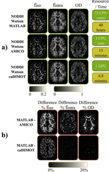
Wefit the NODDI-Watson model to a UK Biobank dataset using three approaches, the NODDI Matlab toolbox (Microstructure Imaging Group - University College London, 2017), AMICO (Daducci et al., 2015) and cuDIMOT. Although Matlab applications are not as optimised as C/Cþþ applications, the only available version of NODDI is implemented in Matlab. Despite this issue, the NODDI toolbox can parallelise thefitting process distributing groups of voxels among several CPU threads. AMICO reformulates the problem as a linear system via convex optimisation and accelerates computations by performing discrete searches in the multi- dimensional space of the problem.Fig. 5a shows maps with the estimated parameters from each approach and the respective execution times. Both cuDIMOT and AMICO achieved accelerations of more than two orders of magnitude compared to NODDI toolbox (cuDIMOT 352x and AMICO 160x) using a single NVIDIA K80 GPU and a single CPU core respectively.
cuDIMOT was 2.2 times faster than AMICO.
To compare the estimates, we treat the NODDI toolbox results as ground truth, and we calculate the percentage absolute difference with the estimates obtained from the other two approaches.Fig. 5b shows higher differences with AMICO than with cuDIMOT for some of the estimated parameters. The differences between the Matlab imple- mentation and cuDIMOT are insignificant, except for the parameterfisoin certain parts of the white matter. However, the values offisoare very low in the white matter, and the absolute difference between the Matlab toolbox and cuDIMOT are very small (~0.003) (See Supplementary Fig. 8). The absolute differences between the Matlab toolbox and AMICO are also small, but more significant (~0.03).
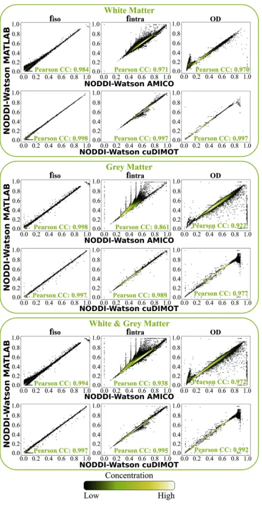
To further explore thesefindings,Fig. 6shows scatterplots of the estimated values throughout the brain. The correlations between the Matlab implementation and AMICO, and between the Matlab toolbox and cuDIMOT are presented. cuDIMOT results are highly correlated to the results from the Matlab tool (Supplementary Fig. 9includes Bland- Altman plots). The discretisation approach used in AMICO is evident in these scatterplots, particularly for thefintraparameter, with discretisation effects. For cuDIMOT, correlations with ground truth is higher. We only find some differences in a few grey matter voxels whereODtakes rela- tively high values (OD>0.85, i.e. very highfibre orientation dispersion).
We compared the distribution of the estimated values for the parameter κ, from whichODis derived (SeeSupplementary Fig. 10a), and we found that for low values ofκ(κ<1), the Matlab toolbox seems to get trapped in a local minimum (κ ¼ 0:5), whereas in cuDIMOT the value of the parameter is pushed towards the lower bound (κ ¼0:0). Moreover, we found that this happens in a very low proportion of voxels located at the interface between grey matter and CSF (SeeSupplementary Fig. 10b). We believe that these differences are due to the numerical approximations used. In the cuDIMOT implementation we approximate the Dawson's integral as in (Press et al., 1988). Likely, the Matlab toolbox is using a different approximation. Overall, these results indicate that cuDIMOT achieves very similar performance to the NODDI Matlab toolbox, and compared with AMICO, cuDIMOT is faster and obtains more accurate results.
We also performed similar comparisons for the NODDI-Bingham model (Microstructure Imaging Group - University College London,
2017). Using a single GPU, cuDIMOT was found to be 7 times faster than the Matlab implementation running on a cluster with 72 cores2(Fig. 7).
We obtain very similar results from both tools; however, the percentage absolute differences (bottom row in Fig. 7) are on average higher compared to the NODDI Watson model. To gain further insight,Fig. 8 shows scatterplots of the parameter values estimated using both methods throughout the brain. In all the parameters, the correlation coefficient was higher than 0.984 in the white matter, and 0.977 in the grey matter.
Notably, we found some voxels where one toolbox returns a very lowDA (near zero) but not the other. We found that these voxels represent a very low proportion of the whole dataset, 0.2%, and they are at the interface between white matter and CSF. We believe that the source of these dif- ferences come from:
Fig. 5.Comparison of three different toolsfitting the NODDI-Watson model. (a) The results from each tool are presented in different rows. Thefirst 3 columns show the map of the estimates for the parametersfiso,fintraand the indexOD. The 4th column shows the employed computational resources and the execution times. (b) Differences, in percentage, of the estimated values between the Matlab toolbox and the other approaches.
2Note the almost sixfold difference between fitting NODDI-Bingham vs.
NODDI-Watson using the Matlab toolbox, despite the higher complexity of NODDI-Bingham. This is due to the inefficient approximation of the confluent hypergeometric function of a scalar argument used in the NODDI-Watson Mat- lab implementation. For this reason, the comparisons in performance gains with cuDIMOT are more meaningful in the NODDI-Bingham case.
Fig. 6. Correlations between the results from NODDI Matlab toolbox and AMICO/cuDIMOTfitting the NODDI-Watson model in the white matter, grey matter and the combination of white&grey matter.
Using a different approximation of the hypergeometric function. In cuDIMOT we use a Saddlepoint approximation (Kume and Wood, 2005) and in the Matlab toolbox the function is approximated as in (Koev and Edelman, 2006).
Different non-linear optimisation method. We use Levenberg- Marquardt whereas the Matlab toolbox uses the active set algorithm included in the fmincon function (Gill et al., 1984).
We also found a few voxels whereDAis estimated with values around 0.5 in cuDIMOT, whereas in the Matlab toolbox the values are different.
This seems to be related to the initial Grid-Search routine and the values that define the grid for the second concentration parameterκ2. Both Matlab toolbox and cuDIMOT reparametrise this parameter asβ ¼κ1 κ2. However, in cuDIMOT we include in the grid a set of values (from 0 to 16), whereas Matlab toolbox uses a single constant value to initialise this parameter, defined by the coefficient between the second and third ei- genvalues of the diffusion tensor. Nevertheless, overall we obtain very high correlations between both toolboxes.
To assess speed-ups achieved by cuDIMOT, we implemented several dMRI models. We report inTable 2the speedups obtained by cuDIMOT using a single NVIDIA K80 GPU, compared to the commonly used tools forfitting these models running on 72 CPU cores, including Cþþand Matlab implementations. A Biobank dataset was used for this experi- ment. We considered the following models:
- Ball&1 stick (Behrens et al., 2003,2007) - Ball&2 sticks
- Ball&1 stick (with gamma-distribution for the diffusivity (Jbabdi et al., 2012))
- Ball&2 sticks (with gamma-distribution for the diffusivity) - NODDI-Watson
- NODDI-Bingham
On average (and excluding NODDI-Watson implementation), using a single GPU cuDIMOT achieves accelerations of 4.3x.
To illustrate theflexibility of cuDIMOT in defining new models, and the benefits from accelerations that allow extensive model comparison, even with stochastic optimisation, we used cuDIMOT to test whether
crossing or dispersing models are more supported by the data. We per- formed a comparison of six diffusion MRI models and used the BIC index for comparing the performance. The models included in this test were:
- Ball&1 stick (with gamma-distribution for the diffusivity (Jbabdi et al., 2012))
- Ball&2 sticks (with gamma-distribution for the diffusivity) - NODDI-Watson
- Ball&racket (Sotiropoulos et al., 2012) - NODDI-Bingham
- NODDI-2-Binghams: we implement an extension of the NODDI- Bingham model (Tariq et al., 2016) for including twofibre orienta- tions with the model signal given by:
Sm¼S0
fisoSisom þ ð1fisoÞ 1ffan2
fintra1Sintra1m þ ð1fintra1ÞSextra1m
þ ð1fisoÞ
ffan2
fintra2Sintra2m þ ð1fintra2ÞSextra2m
(4) Sisom,Sintra1m ,Sintra2m ,Sextra1m andSextra2m are defined as in the NODDI-Bingham model.
The model has a total of 14 free parameters:
Compartments fraction:fiso,ffan2,fintra1,fintra2
Firstfibre distribution:κ1 1,κ1 2,θ1, ϕ1,ψ1
Secondfibre distribution:κ2 1,κ2 2,θ2, ϕ2,ψ2
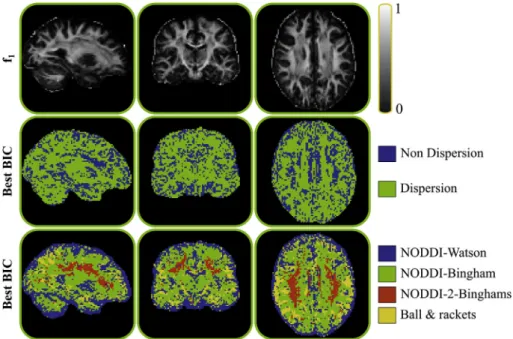
In all cases we ran an initialisation routine (Grid-Search or the output of thefitting process of another model), we run Levenberg-Marquardt and MCMC. cuDIMOT calculates the BIC from the mean of the param- eter estimates. Wefirst classify the six models into two groups, one group with the models that do not characterise the dispersion offibre orien- tations, which include the ball&stick(s) models, and another group with the models that characterise the dispersion. The second row inFig. 9 shows a colour-coded map indicating in what voxels each group gets a better BIC (lower), i.e. its complexity is better supported by the data.
Using dispersion models the diffusion signal is better explained, and the obtained BIC is lower in the majority of brain regions. The last row of Fig. 9compares the four considered dispersion models. The dominant model that gets a lower BIC is NODDI-Bingham (55% of the voxels) followed by NODDI-Watson (24% of the voxels), consistent with the re- sults presented by (Ghosh et al., 2016). Interestingly, 5% of the voxels, particularly in the centrum semiovale, support the existence of dispersing populations crossing each other.
3.2. Tractography with GPUs
In order to validate the GPU-accelerated probabilistic tractography framework we performed various tests and compared the results with the results obtained using a CPU-based tractography application (Smith et al., 2004;Behrens et al., 2007), as implemented in FSL, for both white matter tract reconstruction and connectome generation. Given the sto- chastic nature of probabilistic tractography methods, we expect some variability in the results of both frameworks, but given the high number of samples that we have used in the tests, we expect the results to have converged and the variability to be small. Nevertheless, we run every experiment 10 times and we compare the differences between CPU and GPU results with the run-rerun variability.
Fig. 10a shows some quantitative comparisons of reconstructed tracts using both implementations. We reconstructed 27 major white matter tracts as in (de Groot et al., 2013) (12 bilateral and 3 commissural ones) using standard space tracking protocols and constraints (seeTable 3for a list of reconstructed tracts). In a different test, we generated dense con- nectomes using the HCP grayordinates (91K seed points (Glasser et al., 2013)). To quantify these comparisons, we present the run-rerun vari- ability of each framework independently and the distribution of corre- lation coefficients between the CPU-based and the GPU-based Fig. 7. Comparison of a Matlab tool and cuDIMOTfitting the NODDI-Bingham
model. Thefirst 2 rows show the map of the estimates for the parametersfiso,
fintra, the indicesODandDA, the used computational resources and execution
times for each tool. The bottom row shows the differences, in percentage, of the estimated parameters between the Matlab tool and cuDIMOT.
Fig. 8. Correlations between the results from a Matlab tool and cuDIMOTfitting the NODDI-Bingham model in the white matter, grey matter and the combination of white&grey matter.
Table 2
Speedups obtained by cuDIMOT,fitting several dMRI models to a dataset from the UK Biobank on a single K80 NVIDIA GPU, compared with the commonly used tools that implement these models and executed on a computing cluster using 72 CPU cores (and a single CPU thread per core).
Ball&1-stick
Cþþ
Ball&2-sticks
Cþþ
Ball&1-stickþGamma
Cþþ
Ball&2-sticksþGamma
Cþþ
NODDI Watson Matlab
NODDI Bingham Matlab Common Tools
72 CPU cores
720s 1380s 1260s 2520s 2400m 405m
cuDIMOT single NVIDIA K80
GPU
187s 423s 324s 679s 6.8m 58m
Speedup 3.85x 3.26x 3.88x 3.7x 352x 6.98x
frameworks. In the reconstruction of the 27 tracts the correlation was calculated voxel-wise. In the generation of the dense connectome, the correlation was calculated from all the elements of the connectivity matrix. The individual run-rerun correlation coefficients are higher than 0.999 in all the cases, for both the CPU and the GPU frameworks.
Importantly, the correlation coefficients between CPU and GPU are higher than 0.998, illustrating that the two implementations provide the same solution. Even if these correlations are slightly lower than between the individual run-rerun results (CPU vs. CPU and GPU vs. GPU), this is expected, as some mathematical operations have different implementa- tions (e.g. rounding modes) and different precision in a GPU compared with a CPU (Whitehead and Fit-florea, 2011).Fig. 10b shows a qualita- tive comparison of the reconstruction of six exemplar tracts using both frameworks.
We evaluated the optimal number of CUDA streams (and OpenMP threads) for each test (seeSupplementary Fig. 11). The most efficient configurations were 8 CUDA streams for generating dense connectomes, obtaining a total gain of 1.35x respect using 1 CUDA stream, and 4 CUDA streams for reconstructing tracts, obtaining gains of only 1.12x.Fig. 11a reports computation times reconstructing the 12 bilateral tracts and the 3 commissural tracts individually. A single CPU core was used for running the CPU-based framework, and a single GPU and four CUDA streams for processing the tracts with the GPU-accelerated framework. On average, a speedup of 238x was achieved, in the range of 80x to 357x. In all cases, except for the reconstruction of the Acoustic Radiation (AR), the GPU- based application achieves accelerations of more than two orders of magnitude. In general, if the reconstruction of a tract involves several anatomical constraints that makes the algorithm to stop or discard streamlines at early steps, including tight termination and exclusion masks, the GPU-based framework performs worse, as these masks are not checked until the propagation of the streamlines has completelyfinished (seeSupplementary Fig. 6a). The reconstruction of the Acoustic Radia- tion uses a very tight exclusion mask and thus the achieved performance is lower compared with the reconstruction of other tracts.
Fig. 11b reports the total execution time reconstructing all the tracts.
When the CPU-based tool is used, the reconstruction of several tracts can be parallelised. Tracts are completely independent and thus their reconstruction can be processed by different threads. A total of 27 CPU cores were used in this case, using different CPU threads for recon- structing different tracts. A single GPU and four CUDA streams were used
again for processing the tracts with the GPU-accelerated framework, processing sequentially the different tracts. A speedup of 26.5x was achieved using the GPU-accelerated solution.
We use the CPU-based and the GPU-based frameworks for generating a dense connectome. 91,282 seed points and 10,000 samples per seed point were employed, having a total of 912.82 million streamlines. For generating the connectome with the CPU-based application we used 100 CPU cores, each one propagating 100 streamlines from each seed point.
This process took on average 3.38 h. At the end of the process, the different generated connectomes (on different CPU cores) need to be added. This merging process took on average 6.1 h (due to the size of the final connectivity matrices).
We used 1 single GPU and 8 CUDA streams for generating the con- nectome with the GPU-based application. The process took on average 2.95 h.Fig. 11c reports these execution times and the speedup achieved by the GPU-based framework, with and without considering the merging process required by the CPU multi-core application. Without considering the merging process both applications reported similar execution times.
Considering the merging process, the GPU application was more than three times faster than the CPU multi-core application.
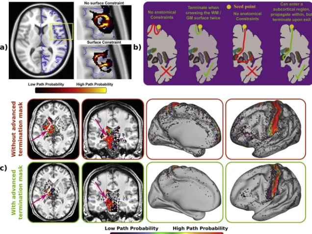
Apart from the computational benefits, we have added new func- tionality to the GPU tractography toolbox. A novel feature is the possi- bility of using surfaces for imposing more accurate anatomical constraints. For instance, we can use a pial surface as termination mask for avoiding the propagation of streamlines outside this surface, and avoiding non-plausible connections along the CSF in the subarachnoid space. As shown in the results ofFig. 12a, surfaces allow us to describe more accurately the cortical folding patterns and allow more accurate constraints to be imposed.
A more sophisticated termination mask mechanism has also been added to the GPU framework. Commonly, termination masks force the algorithm to stop the propagation of the streamlines thefirst time they hit the mask, but sometimes it is reasonable to allow the propagation until certain conditions are met (seeFig. 12b). For instance, to increase the chances of getting“direct”connections, it is desired that a streamline crosses the WM/GM boundary no more than twice when reconstructing cortico-cortical networks, once at the starting point and once at the end point. However, it does not seem plausible to have pathways running in and out of the WM/GM boundary or in parallel along the cortex con- necting several regions. Thus, a special type of termination masks can be Fig. 9. Model performance comparison. Thefirst row shows a map for reference with the estimated fraction of the principalfibre in the ball&2 sticks model. The second and third rows show color-coded maps indicating in what locations a model or a group of models get the best BIC.
used for stopping the streamlines when they cross a surface twice.
Similarly, to encourage direct cortico-subcortical connections, it is un- desirable that a streamline visits several subcortical regions, but ideally we would like a streamline to be able to propagate within a subcortical region. As in (Smith et al., 2012), our framework can use the special
termination masks for stopping the streamlines upon exiting these re- gions, while allowing propagation within them.Fig. 12c shows the effect of imposing these anatomical constraints when generating a dense con- nectome. The special termination mask is defined with a WM/GM boundary surface, and it also includes several subcortical structures Fig. 10. (a) Run-rerun variability of CPU-based and GPU-based probabilistic tractography frameworks and distribution of the correlation coefficients between both frameworks. Results are showed in the reconstruction of 12 bilateral tracts, 3 commissural tracts and in the generation of a dense connectome. Each experiment was run 10 times. The 45 combinations of correlations between re-runs were considered and 45 out of the 100 combinations of CPU vs. GPU correlation coefficients were chosen randomly. (b) Coronal, sagittal and axial views comparing CPU-based and GPU-based frameworks performing probabilistic tractography and reconstructing some major white matter tracts. Each colour represents a different white matter tract. These paths are binarised versions of the path distributions after being thresholded at 0.5%.
(accumbens, amygdala, caudate, cerebellum, hippocampus, pallidus, putamen and thalamus). The connectivity pattern from the sensori-motor part of the thalamus without and with advanced termination masks is illustrated. In the former case, the streamlines can cross the cortex or subcortical structures several times and continue propagating, generating a number of false positives (for instance see hotspots along the frontal medial surface). In the latter case, this situation is avoided, and a more realistic connectivity map is obtained, connecting the sensorimotor part of the thalamus to sensorimotor cortical regions.
Given the speed and facility to run-rerun probabilistic tractography using the developed GPU toolbox, we performed a convergence study.
We evaluated the number of samples that are needed per seed point when generating a dense connectome in order to achieve convergence. To do that, we generated a dense connectome multiple times using a different number of samples per seed point. Fig. 13shows the correlation co- efficients with respect to an assumed converged dense connectome, which was generated using 100,000 samples per seed. Thefigure also shows the correlation coefficients between consecutive runs in terms of number of samples per seed. It seems that even with 1000 samples and 18 min run, the results are almost converged. Using 10,000 samples per seed achieves convergence, while the time for generating the con- nectome is still reasonable, less than 3 h using a single GPU.
4. Discussion
We have presented GPU-based parallel computational frameworks for accelerating the analysis of diffusion MRI, spanning from voxel-wise biophysical modelfitting to tractography and whole-brain connectome generation. Despite the difference in the inherent parallelisability of these applications, GPUs can offer considerable benefits when challenges are carefully considered. Performances similar to 200 CPU cores were achieved using a single GPU, which change the perspective of what is
computationally feasible. The GPU toolboxes will be publically released as part of FMRIB's Software Library (FSL).
The accelerations achieved by the designs proposed here can be tremendously beneficial. Big databases arise more and more often from large consortiums and cornerstone projects worldwide. Hundreds or even thousands of datasets need to be processed. The throughput of the par- allel designs using a single or a multi-GPU system is higher than a CPU multi-core system. Very large recent studies such as the Human Con- nectome Project (HCP) (Van Essen and Ugurbil, 2012;Van Essen et al., 2012;Sotiropoulos et al., 2013), (data from 1200 adults), the Developing Human Connectome Project (dHCP) (data from 1000 babies) and UK Biobank (Miller et al., 2016;Alfaro-Almagro et al., 2018) (data from 100, 000 adults) are using our parallel designs for processing these datasets on GPU clusters. For instance, a 10-GPU cluster has been built for processing the most computationally expensive tasks of the UK Biobank pipeline.
The cluster allowsfitting the ball&sticks model to 415 datasets per day.
Running the same tasks with a cluster of 100 CPU cores, only 25 datasets could have been processed per day. Moreover, to obtain a similar throughput as the 10-GPU cluster, more than 1600 CPU cores would have been necessary. Nevertheless, there are cloud computing platforms that provide on-demand computational resources, including GPUs. Recent studies have presented the pros and cons of using these services for running neuroimaging applications, including cost comparisons (Mad- hyastha et al., 2017).
We made a price-performance comparison between the multi-CPU and single-GPU configurations, i.e. assessed the relative performance gains of the GPU designs per unit cost. Indicative costs are detailed in Supplementary Table 1, suggesting a price of ~£10800 for 72 CPU cores
and£4960 for a dual GPU (K80). It should be noted that these prices
reflect a GPU and CPU model and can change depending on choice and generations. They however reflect reasonably the current costs. On average, cuDIMOT on a single GPU (and single CPU core) was 4.3x faster than 72 CPU cores. Thus, in terms of price-performance ratio the parallel solution on a single GPU offers 17.6 times better speedup/pound than the 72 CPU core system. For generating a dense connectome, the GPU system had a total cost of£3680 (a single GPU and 8 CPU cores) and was 3.2x faster than 100 CPU cores, offering 13.04 times better speedup/pound.
Apart from increasing feasibility in big imaging data exploration, the designs presented here can assist in model exploration and development, as estimation and testing is an inherent part of model design. Moreover, the response time for analysing a single dataset is dramatically reduced from several hours/days to few minutes using a single GPU, and close to real-time processing could make these methods more appealing for clinical practice.
4.1. GPU-based biophysical modelling
We have presented a generic modelling framework, cuDIMOT, that provides a model-independent front-end, and automatically generates a GPU executablefile that includes severalfitting routines for user-defined voxel-wise MRI models. Although parallel designs for processing MRI voxel-wise applications are straightforward, for instance creating as many threads as voxels, challenges need to be considered for achieving efficient solutions on GPUs. Here we have proposed a second level of parallelisation where the most expensive within-voxel tasks are distrib- uted amongst threads within a CUDA warp. We have used cuDIMOT to explore diffusion models that characterisefibre orientation dispersion, and we have shown that it can be very useful for exploring, designing and implementing new dMRI protocols and models. It is easy to use and generates very efficient GPU-accelerated solutions.
Some toolboxes with the same purpose as cuDIMOT have been recently presented (Harms et al., 2017;Fick et al., 2018). In (Fick et al., 2018) a python generic toolbox forfitting multi-compartments dMRI models is proposed, but it does not include any parallelisation strategy. In (Harms et al., 2017) a toolbox for parallelising the optimisation routines is proposed. Even if the initial version did not include the option for Table 3
List of reconstructed tracts sorted by number of propagated streamlines. Different number of seed points and samples are used for reconstructing the tracts. Some tracts have a bilateral homologue (þ) and some others no ().
Tract Name Acronymic Number of seeds
Samples per seed
Number of streamlines
Left/
Right Uncinate
fasciculus
UNC 1692 1200 2,030,400 þ
Medial lemniscus ML 1926 1200 2,311,200 þ
Corticospinal tract
CST 723 4000 2,892,000 þ
Anterior thalamic Radiation
ATR 3181 1000 3,181,000 þ
Parahippocampal part of cingulum
PHC 1887 3000 5,661,000 þ
Middle cerebellar peduncle
MCP 2075 4400 9,130,000 –
Forceps major FMA 18,159 600 10,895,400 –
Inferior longitudinal fasciculus
ILF 9207 1200 11,048,400 þ
Forceps minor FMI 19,195 600 11,517,000 –
Superior longitudinal fasciculus
SLF 32,831 400 13,132,400 þ
Superior thalamic radiation
STR 21,019 800 16,815,200 þ
Cingulate gyrus part of cingulum
CGC 1137 20,000 22,740,000 þ
Inferior fronto- occipital fasciculus
IFO 15,412 4400 67,812,800 þ
Posterior thalamic radiation
PTR 3669 20,000 73,380,000 þ
Acoustic radiation AR 23,105 10,000 231,050,000 þ
performing stochastic optimisation or the ability to add priors on the model parameters, an MCMC routine has been very recently included (Harms and Roebroeck, 2018). It is implemented in a more generic (non-GPU specific) programming model (OpenCL (Stone et al., 2010) rather than CUDA), allowing the parallelisation on both multi-core CPUs and GPUs, but potentially achieving lower performance on NVIDIA GPUs as some type of instructions can differ in the implementation. For instance, CUDA Shuffle instructions (NVIDIA, 2014a), which are used in cuDIMOT kernels (see implementation details in the Supplementary material), allow sharing data between threads within a warp and offer performance improvement, but are not supported in OpenCL (Khronos OpenCL Working Group, 2012), where same results must be achieved with slower operations. Therefore, it is expected that CUDA imple- mentations on NVIDIA GPUs will be more efficient than OpenCL
counterparts, this however remains to be tested explicitly for our design.
It would be of interest for future work to directly compare the two implementations.
Our framework offers a C-like interface. We are planning as a future extension to design an even more user-friendly Application Programming Interface (API) and a python parser to communicate this API with cuDIMOT.
Our toolbox has been designed for processing datasets with any number of voxels and measurements. If the memory required for storing the data of all the voxels exceeds the device memory, the framework divides the data into several subsets (according to the amount of device memory available), and these subsets are processed one after the other.
However, before being processed, each subset needs to be copied into device memory. This can create a performance penalty if the device Fig. 11. (a) Execution times (in logarithmic scale) and speedup (standard deviationσis also shown) in the reconstruction of 12 bilateral tracts and 3 commissural tracts comparing a GPU-based with a CPU-based probabilistic tractography framework. (b) Execution times (in logarithmic scale) and speedup (and its standard deviationσ) reconstructing a total of 27 tracts and (c) generating a dense connectome, comparing a single GPU with several CPU cores.