Adversarial Robustness of Linear Models:
Regularization and Dimensionality
István Megyeri1, István Hegedűs1 and Márk Jelasity1,2 ∗
1- University of Szeged, Hungary
2- MTA-SZTE Research Group on Artificial Intelligence, Hungary
Abstract. Many machine learning models are sensitive to adversarial input, meaning that very small but carefully designed noise added to cor- rectly classified examples may lead to misclassification. The reasons for this are still poorly understood, even in the simple case of linear models.
Here, we study linear models and offer a number of novel insights. We focus on the effect of regularization and dimensionality. We show that in very high dimensions adversarial robustness is inherently very low due to some mathematical properties of high-dimensional spaces that have received lit- tle attention so far. We also demonstrate that—although regularization may help—adversarial robustness is harder to achieve than high accuracy during the learning process. This is typically overlooked when researchers set optimization meta-parameters.
1 Introduction
The high sensitivity of most machine learning models to adversarial examples was pointed out not long ago [1, 2]. A number of methods have been proposed to create better adversarial examples [3, 4] as well as to provide defense mechanisms against these [5, 6].
Here, we focus on the adversarial robustness of linear machine learning mod- els. The theoretical basis of the problem is still lacking. Some results are known e.g. Fawzi et al. [7] offer bounds on robustness for the linear case based on the distance of classes, but their study is orthogonal to ours. Goodfellow at al. [1]
suggested that higher-dimensional linear models are more sensitive because the same amount of noise in each dimension can result in a larger Euclidean distance from the point simply due to the larger number of dimensions, provided the sign of the noise is the same as the sign of the value in the given dimension. However, we argue that the Euclidean distance is of limited interest simply because classes and data points in general will also have larger Euclidean distances from each other in higher dimensions.
In this paper, we propose novel insights, which provide an alternative expla- nation to the adversarial sensitivity of linear models. We focus on the effect of regularization and dimensionality. We will show that in very high dimensions adversarial robustness is inherently very low due to the fact that a random hy- perplane is very close to any data point. This property which has received little attention so far, is highly counter-intuitive.
∗This study was supported by the National Research, Development and Innovation Of- fice of Hungary through the Artificial Intelligence National Excellence Program (grant 2018- 1.2.1-NKP-2018-00008) and by the Hungarian Ministry of Human Capacities (grant 20391- 3/2018/FEKUSTRAT).
We also point out that regularization has a profound effect on adversarial robustness. From the point of view of prediction accuracy and adversarial ro- bustness the amount of regularization required will be different. We should add that the current practice of setting meta-parameters based only on prediction accuracy might result in very high sensitivity to adversarial examples. This is because the convergence of robustness is much slower than that of accuracy and because robustness requires stronger regularization.
We shall also provide a thorough experimental evaluation of our claims where we study the effect of dimensionality, regularization, and the interaction of these two factors. In this evaluation, we will use artificial datasets as well as a subset of the MNIST dataset.
2 Linear Models in High Dimensional Spaces
We are given a set of training instances of the form (x, y), x∈Rn, y ∈ {0,1}, and we are looking for a hyperplaneP l(w) ={z|hw, zi= 0} defined byw∈Rn such that P l(w)separates the data points with different labels. This plane is typically found via optimizing a loss function based on the examples and w.
Model optimization typically starts with a random initial model, or, equiva- lently, an initial model that is independent of the optimal model. The following result implies that such a random model will be extremely close to any point in expectation, hence, it should also be very close to each instance. This highly unintuitive property implies that a random plane has a very high sensitivity to adversarial examples.
Proposition. Let w∈Rn define a random plane P l(w) ={z|hw, zi= 0}. Let wi(i= 1, . . . , n)be i.i.d. random variables withP(wi=−1) =P(wi= 1) = 0.5.
Let d(1, P l(w))denote the distance betweenP l(w)and the point 1= (1, . . . ,1).
Then we have limn→∞E(d(1, P l(w))) =O(1).
Proof. We have d(1, P l(w)) = |h1, wi|/kwk2 = √1n|Pn
i=1wi|. Also, we have Pn
i=1wi→√nN(0, σ2)due to the central limit theorem, whereσ2= 0.25is the variance of wi. The mean of |N(0, σ2)| is finite and it does not depend on n, so it isO(1); thus E(√1n|Pn
i=1wi|)→ √1n
√nO(1) =O(1), which completes the proof.
Note that there exists a plane for which the distance from1is√n=O(√n), namely whenw =1. However, according to the result above, a random plane is of distance O(1) in expectation. The result is not specific to 1 because it is invariant to rotation. The striking consequence is that a random plane will result in a high sensitivity to adversarial examples, no matter how the classes are positioned. This means that the optimal plane in terms of distance is very special, regardless of the difficulty of the classification problem, so we suspect that this very special plane is hard to find during optimization. Our experimental results are consistent with this view.
3 Linear Models and Regularization
Here, we argue that regularization is closely related to the geometric properties outlined in Section 2. Assuming n examples(xi, yi), xi ∈Rn, yi ∈ {0,1}, i= 1, . . . , n, let us now consider logistic regression where the goal is to approximate the data using the logistic function y ≈σ(wTx+b) = 1/(1 +e−wTx+b). This will lead to a linear separator defined by w and b and a logistic probability approximation as a function of the distance from the separating hyperplane.
The loss function typically used to find the best model (that is, w and b) is the negative log likelihood function L(w, b) = −Pn
i=1yi·log(σ(xi;w, b)) + (1−yi)·log(1−σ(xi;w, b)). To handle noisy data, it is customary to add a regularization term to the loss function. Here we focus on the so-called L2 regularization: L(w, b) +αkwk22, where αis the regularization coefficient.
We would like to study the effect of regularization from the point of view of adversarial robustness. L2 regularization results in preventing the length of w from growing indefinitely. This in turn results in preventing the derivative of the model from growing indefinitely. To see this, consider the derivative σ(a·x)′ =aσ(a·x)σ(1−a·x). Clearly, increasing the length ofwwill make the logistic curve steeper. Without regularization, the model in practice becomes a step function so the loss function will simply attempt to minimize the number of misclassified examples. With regularization, all the examples will affect the orientation of the separating hyperplane.
This means that if regularization is not strong enough then noisy examples will have too much influence, forcing the hyperplane out of optimal position, which in turn will result in very high adversarial sensitivity according to the proposition provided in Section 2. Accordingly, we expect that for optimal ro- bustness one will have to use quite strong regularization.
4 Experimental Results
In order to evaluate the effect of dimensionality and regularization, we carried out a systematic experimental study. Now let us describe the experimental setup and the methodology in detail.
4.1 Binary Classification Problems
We will use two binary classification problems that are described below. The first dataset is a subset of the MNIST dataset [8] that includes two classes: 3 and 7 (also used by the authors of [1]). We will refer to this dataset asMNIST-73. It contains about 6000 samples per class. The raw pixel values were normalized to the range[0,1].
We will also use an artificial dataset called 2-Gauss. The two classes are defined by the distributionsN(1,Σ)andN(0,Σ), where0is the origin andΣis the diagonal matrix4I, hence the variance isσ2= 4, which is the same for each dimension. Note that the Euclidean distance of the class centers is√n, wheren is the dimension. Here, we sampled 6000 instances per class.
For each dataset, 100/6 ≈16.7% of the data was separated to form a test set. In the preprocessing step, the training data values were translated so as to
have a zero mean. The mean was estimated over the training set, and the test set was translated as well using this value.
To examine the effect of the dimensionality on adversarial robustness, we will use a range of input dimensions. The dataset 2-Gauss can naturally be generated in any dimensions. The MNIST-73 examples were scaled using im- age processing algorithms. The original dimension of the images was 28×28.
We performed preliminary tests with different interpolation methods (cubic, lin- ear, nearest-neighbor) that gave similar results. Here, we applied the nearest- neighbor method.
4.2 Methodology
Our two main measures of interest areaccuracy (i.e. the proportion of correctly classified examples) and the distance of the examples from the hyperplane nor- malized by the dimension √
n. The latter measure characterizes the sensitivity to adversarial examples; namely the smaller the distance, the higher the sensi- tivity. Here, we normalize the distance by√nfor two reasons. First, it is more meaningful to measure sensitivityrelativeto the distance of the two classes, and the distance of the two classes grows with √n. Second, in the case of image data, this also means that we characterize the sensitivity of each pixel, which is a more natural measure. We will call this measure thenormalized distance.
We used ADAM [9] as our optimizer with a minibatch size of 32. Since we were interested in the actual optimal model (to avoid artifacts due to early stopping) we ran the algorithm with an extremely small stopping threshold of 10−10. We will also include results with a10−4stopping threshold that is often used as a default. We can still study the effect of early stopping, since we record the convergence history as well. In our plots, we will indicate the regularization coefficient used in the case ofn= 28×28, however, for different dimensionalities, the regularization value was scaled proportional to n to make the strength of regularization in different dimensions comparable.
4.3 Results
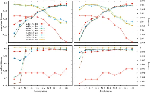
Figure 1 shows some of the results of our experiments. The MNIST-73results indicate that normalized distance and accuracy behave very differently in terms of regularization. Most importantly, one is normally interested in prediction performance, and the meta-parameters optimal for that purpose perform rather badly for adversarial robustness. To optimize the distance, it is good to have a regularization coefficient that is as large as possible, whereas accuracy displays a degrading trend with increased regularization. These observations hold true regardless of the problem dimension. In other words, in each dimension we see that they have almost the same values.
The2-Gaussproblem behaves slightly differently because no noisy examples are added and because in high dimensions there is a wide linear separation mar- gin between the classes and this grows with n. The optimal values for distance and accuracy are found in almost every case. However, we noticed that for low regularization values the optimizer struggles to find the optimum in high dimen- sions. For no regularization, even the smaller stopping threshold is insufficient
0 0.02 0.04 0.06 0.08 0.1
0 1e-4 5e-4 1e-3 5e-3 1e-2 5e-2 1e-1 5e-1 1e0
normalized distance
n=10×10, dist n=18×18, dist n=28×28, dist n=36×36, dist n=10×10, acc n=18×18, acc n=28×28, acc n=36×36, acc
0 1e-4 5e-4 1e-3 5e-3 1e-2 5e-2 1e-1 5e-1 1e0 0.945 0.95 0.955 0.96 0.965 0.97 0.975 0.98 0.985 0.99 0.995
accuracy
0.25 0.3 0.35 0.4 0.45 0.5
0 1e-4 5e-4 1e-3 5e-3 1e-2 5e-2 1e-1 5e-1 1e0
normalized distance
Regularization
0 1e-4 5e-4 1e-3 5e-3 1e-2 5e-2 1e-1 5e-1 1e0 0.991 0.992 0.993 0.994 0.995 0.996 0.997 0.998 0.999 1
accuracy
Regularization
Fig. 1: Normalized distance and accuracy as a function of regularization coeffi- cient and dimension for the MNIST-73dataset (top) and the 2-Gaussdataset (bottom), and stopping threshold10−4 (left) and10−10 (right).
to find the theoretically optimal model. This is because then the loss function is extremely flat. This effect is closely related to the dimensionalityn, and the problem is more severe with larger values ofn.
Let us also examine the dynamics of convergence during optimization, which is shown in Figure 2. Clearly, the convergence of distance is significantly slower than that of accuracy in each case. For the2-Gaussproblem, this effect is more marked. Withα= 10−4, due to the wide separation margin and relatively large weights, the loss function practically vanishes and gives only a very weak signal to the optimizer, while the accuracy attains its optimum quite quickly.
With the MNIST-73 dataset we see there is a local optimum for distance when no regularization is applied. This is due to the length of the parameter vector w gradually increasing. With the 2-Gauss dataset we have no noisy examples that could make the model go in the wrong direction aswgrows due to the lack of regularization, so this effect is not so marked.
5 Conclusions
In this study, we demonstrated that even in the case of simple binary classifica- tion problems with linear models, the adversarial problem is real and it strongly depends on regularization and the less obvious properties of high-dimensional spaces. We presented an experimental evaluation where we showed that the optimal regularization strength is very different for adversarial robustness and prediction accuracy, and that the convergence of adversarial robustness is much slower than that of the accuracy metric. Also, in higher dimensions an overly
0 0.2 0.4 0.6 0.8 1
1 10 100 1000 10000
accuracy/loss
α = 10-4
1 10 100 1000 0
0.01 0.02 0.03 0.04 0.05 0.06 0.07 0.08 0.09
normalized distance
α = 10-1
0 0.2 0.4 0.6 0.8 1
1 10 100 1000 10000
accuracy/loss
Updates
test accuracy train accuracytest distance train distancetrain losstest loss
1 10 100 1000 0
0.05 0.1 0.15 0.2 0.25 0.3 0.35 0.4 0.45 0.5
normalized distance
Updates
Fig. 2: Convergence of normalized distance and accuracy inn= 28×28dimen- sions for theMNIST-73 dataset (top) and the2-Gaussdataset (bottom), with regularization coefficientα= 10−4(left) andα= 10−1(right).
weak regularization setting might result in a significantly harder optimization problem in some cases.
References
[1] Ian J. Goodfellow and Jonathon Shlens Christian Szegedy. Explaining and harnessing adversarial examples. In3rd Intl. Conf. on Learning Representations (ICLR), 2015.
[2] Christian Szegedy, Wojciech Zaremba, Ilya Sutskever, Joan Bruna, Dumitru Erhan, Ian J.
Goodfellow, and Rob Fergus. Intriguing properties of neural networks. In2nd Intl. Conf.
on Learning Representations (ICLR), 2014.
[3] Seyed-Mohsen Moosavi-Dezfooli, Alhussein Fawzi, and Pascal Frossard. Deepfool: A simple and accurate method to fool deep neural networks. InThe IEEE Conf. on Computer Vision and Pattern Recognition (CVPR), pages 2574–2582, June 2016.
[4] Nicholas Carlini and David A. Wagner. Towards evaluating the robustness of neural net- works. In2017 IEEE Symposium on Security and Privacy, SP 2017, San Jose, CA, USA, May 22-26, 2017, pages 39–57. IEEE Computer Society, 2017.
[5] Aleksander Madry, Aleksandar Makelov, Ludwig Schmidt, Dimitris Tsipras, and Adrian Vladu. Towards deep learning models resistant to adversarial attacks. In6th Intl. Conf.
on Learning Representations (ICLR), 2018.
[6] Florian Tramer, Alexey Kurakin, Nicolas Papernot, Ian Goodfellow, Dan Boneh, and Patrick McDaniel. Ensemble adversarial training: Attacks and defenses. In 6th Intl.
Conf. on Learning Representations (ICLR), 2018.
[7] Alhussein Fawzi, Omar Fawzi, and Pascal Frossard. Analysis of classifiers’ robustness to adversarial perturbations. Machine Learning, 107(3):481–508, Mar 2018.
[8] Yann Lecun, Léon Bottou, Yoshua Bengio, and Patrick Haffner. Gradient-based learning applied to document recognition. Proc. of the IEEE, 86(11):2278–2324, November 1998.
[9] Jimmy Ba and Diederik Kingma. Adam: A method for stochastic optimization. In3rd Intl. Conf. on Learning Representations (ICLR), 2015.