Új irányzatok a hulladékégető erőművek megbízhatósági, rendelkezésre állási és karbantartási optimalizálásában

(1)

(2)

N N E E W W T TR RE EN ND D S S I IN N R RE E L L IA I AB BI IL LI IT TY Y, , AV A V AI A IL LA AB BI IL LI IT TY Y A AN N D D M MA AI IN NT TE EN NA AN N C C E E OP O P TI T IM MI I S S A A TI T IO ON N O OF F W WA AS ST TE E T TH HE ER RM MA AL L

T T R R E E A A T T M M E E N N T T P P L L A A N N T T S S

P P h h D D T T h h e e s s i i s s

Supervisor

2010

(3)

ii

NEW TRENDS IN RELIABILITY, AVAILABILITY AND MAINTENANCE OPTIMISATION OF WASTE THERMAL TREATMENT PLANTS

Értekezés doktori (PhD) fokozat elnyerése érdekében Írta:

Készült a Témavezető

Elfogadásra javaslom (igen / nem)

...

(aláírás) A jelölt a doktori szigorlaton ... %-ot ért el,

Az értekezést bírálóként elfogadásra javaslom:

Bíráló neve: ... igen / nem

...

(aláírás) Bíráló neve: ... igen / nem

...

(aláírás) Bíráló neve: ... igen / nem

...

(aláírás) A jelölt az értekezés nyilvános vitáján ... %-ot ért el

Veszprém,

...

a Bíráló Bizottság elnöke A doktori (PhD) oklevél minősítése: ...

...

Az EDT elnöke

(4)

iii

LIST OF TABLES

Table 1.1 Affect of complexity to the reliability of series equipment. ... 7

Table 1.2 Comparison of availability values and corresponting downtimes. ... 8

Table 3.1 Major aspects to perform software tools assessment... 35

Table 3.2 Some availability packages and related software tools. ... 42

Table 3.3 Specific reliability packages and related software tools. ... 43

Table 3.4 General comparison of reliability software candidates. ... 58

Table 5.1 Software groups to choose candidates from. ... 70

Table 5.2 Main system components. ... 76

Table 6.1 Equipment units, subsystems, energy and material streams of the plant. ... 84

Table 6.2 Provided RAM measures of the plant. ... 87

Table 6.3 Calculated RAM measures of the plant. ... 87

Table 6.4 Main characteristics of the subsystem as the output of the performed analyses. ... 90

Table 6.5 Input values. ... 91

Table 6.6 Maintainability of the subsystem. ... 93

Table 6.7 Simulation results of experiment #1. ... 96

Table 6.8 Simulation results of experiment #2. ... 98

(9)

viii

LIST OF FIGURES

Figure 1.1 The difference between failure, fault, and error. ... 4

Figure 1.2 Series system configuration. ... 4

Figure 1.3 Parallel system configuration. ... 5

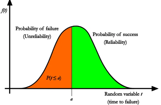
Figure 1.4 Reliability represented as the area under the probability density function. ... 16

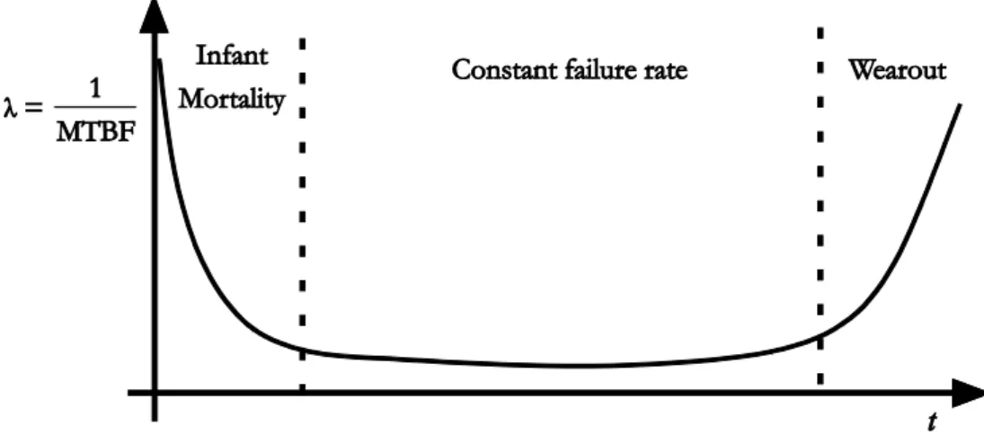
Figure 1.5 Typical bath curve of hardware failures. ... 17

Figure 2.1 Waste management hierarchy. ... 29

Figure 3.1 Relationship between fault tree and RBD. ... 34

Figure 3.2 Schema of a simple RBD. ... 37

Figure 3.3 A typical fault tree diagram. ... 38

Figure 3.4 Fault tree, RBD, equations and their relationship in series systems. ... 38

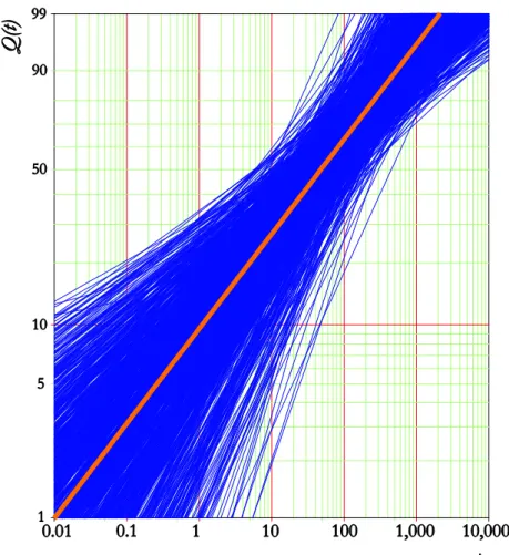
Figure 3.5 Simulation of unreliability in SimuMatic, a Weibull++ extension. ... 41

Figure 3.6 Working screen of Relex Reliability Studio. ... 47

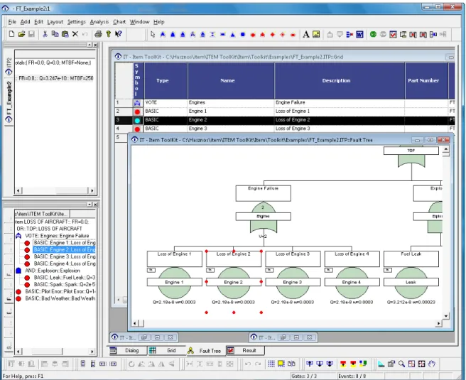
Figure 3.7 Editing a Fault Tree in ITEM Toolkit. ... 49

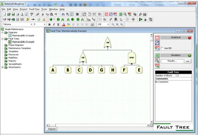
Figure 3.8 A Fault Tree in ReliaSoft BlockSim. ... 52

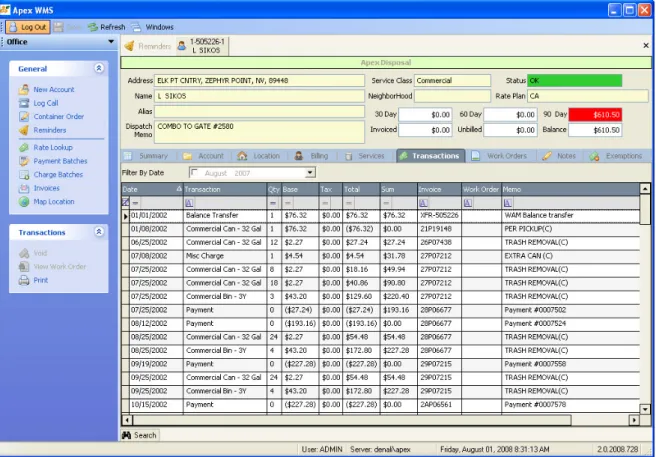
Figure 3.9 Working screen of Apex WMS. ... 54

Figure 3.10 Precision and other settings in LINGO. ... 56

Figure 3.11 Graphical user interface of MPL for Windows. ... 57

Figure 5.1 Combination of software. ... 70

Figure 5.2 Flowchart of the methodology. ... 71

Figure 5.3 Scheme of waste management system tree. ... 75

Figure 5.4 Availability diagram of the major parts of waste management chains. ... 77

Figure 5.5 RBD of a waste management system. ... 78

Figure 6.1 Technological scheme of the plant Termizo. ... 83

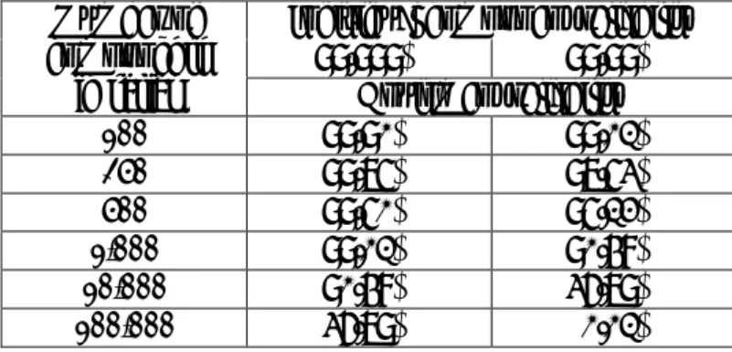
Figure 6.2 Fault tree diagram and fault tree table of Termizo. ... 85

Figure 6.3 Downtimes (DT) and uptimes (UT) of the plant. ... 86

Figure 6.4 RBD of Termizo. ... 88

Figure 6.5 Effects of fouling in the plant. ... 89

Figure 6.6 Technological scheme of the subsystem. ... 90

Figure 6.7 The manually extended fault tree diagram and fault tree table. ... 91

(10)

ix

Figure 6.8 Fault tree diagram and fault tree table modules in Relex Reliability Studio... 92

Figure 6.9 Maintainability results. ... 94

Figure 6.10 SOFC flowsheet of the case study. ... 95

Figure 6.11 Grand composite curve of SOFC integration. ... 95

Figure 6.12 HEN topology. ... 96

Figure 6.13 Fault tree table and diagram of the case study. ... 97

(11)

x

KIVONAT

A disszertáció a szerző doktoranduszi kutatási tevékenységét és annak eredményeit mutatja be. A kutatás eredeti célja (nevezetesen a hulladékkezelő rendszerek megbízhatóságának szoftveres modellezéséhez és optimalizálásához való tudományos közreműködés) megvalósult.

Ezzel egyidőben hőcserélő hálózatok hasonló kérdései is elemzésre kerültek, hiszen ezen rendszerek gyakori alrendszerei a különféle ipari folyamatoknak, beleértve a hulladékégetést és a szennyvíz-kezelést is. A kutatás részeként így megvizsgálásra kerültek a komplex megbízható- sági szoftverek alkalmazási lehetőségei hőcserélő hálózatok modellezésében és optimalizálásá- ban. A területen új szoftveres módszertan is bevezetésre került.

Az energiatermelés és potenciális energiamegtakarítás megbízhatósági kérdéseinek jelentős hatásai figyelemre méltó modelleket generáló, hatékony szoftvereszközök implementálásával értékelhetők ki. Ezen eszközök ráadásul szemléletes formában jelenítik meg a kimenetet, táblá- zatos és/vagy grafikus formában.

Bár sokféle szoftvertípus létezik, melyek hasznosak lehetnek a hulladékkezelés megbízható- ságának modellezésében, számos probléma meglehetősen bonyolulttá teszi a kérdést. Alapos kiértékelés és minősítés után egyértelművé vált, hogy sem a specifikus hulladékkezelő szoftver- eszközök, sem az összetett megbízhatósági szoftverek nem képesek önmagukban megfelelő modellezési-optimalizálási környezetet biztosítani. Ez a felismerés vezetett egy új szoftveres módszertan kidolgozásához (a különféle szoftvertípusok képességeinek kombinálása érdeké- ben). A folyamat nem volt következetesen előremutató, de végül siker koronázta. Számos elő- nyös tulajdonságot sikerült azonosítani és azokat ipari esettanulmányokkal bizonyítani.

A megbízhatósági elemzések új módja került bevezetésre, mely azt is definiálja, hogy mi- ként lehet az eredményeket felhasználni a karbantartási műveletek hatékonyságának növelé- sére. Ez a módszer a rendszer-megbízhatóságot optimálisabbá teszi.

A kutatás fő célja különféle számszerűsített teljesítmény-mutatók megbízhatósági számítá- sokkal, becslésekkel, jóslásokkal és szimulációkkal történő meghatározásaként foglalható össze. Ezen mutatók közül a legfontosabb a rendelkezésre állás, a karbantarthatóság, az elvárt működésen kívül eltelt idő, az előforduló hibák száma, valamint a teljes rendszerköltség. Ezek kiértékelése fontos szerephez jut az optimális döntéshozatalnál. A rendszer-konstrukciónak maximalizálnia kell a tisztább és hatékonyabb feldolgozáshoz vezető rendszer-teljesítményt, ugyanakkor minimalizálnia kell a rendszer összköltségét a megengedett korlátokon belül.

A korszerű szoftvereszközök elősegíthetik a megbízhatóságért felelős mérnökök munkáját ezen célok elérésében.

(12)

xi

ABSTRACT

The presented work describes the PhD research and results of the Author in reliability, availability and maintenance optimisation. Due to some unsolved problems identified in waste management reliability, research has been conducted. The main part of the research is a contribution to software support for modelling and optimising reliability issues of waste management systems. In addition, similar issues involving heat exchanger networks were investigated. They are often subsystems of industrial processes, including thermal treatment of waste and waste water treatment. Part of the research involved the investigation of RAM software potentials in modelling and optimising heat exchanger networks. A new methodology was suggested in this field.

The considerable effect of reliability issues on energy generation and potential energy saving can be assessed by implementing effective software tools generating impressive models.

They also provide output visualization via a tabular and/or graphical representation.

Although there are many software groups that can be useful in waste management reliability modelling, several problems make the field quite complex. After extensive software evaluation and assessment it was realized that neither specific waste management software tools nor comprehensive reliability software packages are capable to provide adequate modelling and optimisation environment individually. Consequently, a new software methodology was developed that combines the capabilities of various software groups. Several advantages were identified and proved through industrial and demonstrative case studies.

A new method was defined to conduct reliability analyses and apply the results to improve the efficiency of maintenance actions. This leads system reliability towards optimality.

The main goal can be described as providing quantitative forecasts of various performance measures of waste management systems through reliability calculations, estimations, predictions and simulations. Such measures are availability, reliability, maintainability, downtimes, number of failures, and overall system cost. The evaluation of these measures is important for optimal decision making. The system design should both maximise the system performance leading to cleaner and more effective processing and minimise the overall cost within the allowable constraints.

Modern software tools are capable to assist reliability engineers to reach these goals.

(13)

xii

ZUSAMMENFASSUNG

Die vorliegende Dissertation stellt die PhD-Forschungstätigkeit des Verfassers und die Ergebnisse dieser Tätigkeit dar. Die originale Zielsetzung (nämlich die wissenschaftliche Mitarbeit bei der Modellierung mit Software und der Optimalisierung der Verlässlichkeit von Systemen für Abfallwirtschaft) verwirklichte sich. Zur gleichen Zeit wurden auch ähnliche Fragen der Wärmeaustausch-Systemen analysiert, da diese Systeme auch als Untersysteme von verschiedenen Industrieprozessen, z.B. der Müllverbrennung und der Abwasserbeseitigung häufig erscheinen. Während der Forschung wurden so die Verwendungsmöglichkeiten der komplexen Verlässlichkeitssoftwares durch Modellierung und Optimalisierung von Wärme- austausch-Systemen untersucht. In diesem Bereich wurde auch eine neue Softwaremethodik eingeführt.

Die bedeutenden Wirkungen der Verlässlichkeitsfragen der Energieproduktion und der potentiellen Energiesparung können mit Implementierung wirksamer Softwaremittel ausgewertet werden, die beachtungswerten Modellen generieren. Diese Mittel zeigen sogar den Ausgang in anschaulicher Form, d.h. tabellarisch und/oder in graphischer Form.

Zwar es vielerlei Softwaretypen gibt, die in der Modellierung der Verlässlichkeit der Abfall- handlung sehr gut zur Hand kommen, machen einige Probleme die Frage kompliziert. Nach gründlicher Auswertung und Qualifizierung wurde es eindeutig, dass weder die spezifischen Softwaremittel für die Abfallwirtschaft noch die komplexe Verlässlichkeitssoftware dazu fähig sind, selbst einen entsprechenden Umkreis für die Modellierung und Optimalisierung zu sichern. Diese Erkennung führte zur Ausarbeitung einer neuen Softwaremethodik (im Inter- esse der Kombinierung der Fähigkeiten der verschiedenen Softwaretypen). Der Prozess war nicht konsequent vorwärts weisend, aber er war von Erfolg begleitet. Es gab zahlreiche vor- teilhafte Eigenschaften, die auch mit industriellen Fallstudien bewiesen wurden.

Eine neue Art der Verlässlichkeitsanalysen wurde eingeführt, die auch definiert, wie die Ergebnisse für die Steigerung der Wirkung der Wartungsoperationen angewandt werden können. Mit dieser Methode wird die Systemverlässlichkeit optimaler.

Das Hauptziel der Forschung kann als verschiedene numerische Leistungskennziffer zusammengefasst werden, die durch Verlässlichkeitsrechnungen, Schätzungen, Voraussagen und Simulationen bestimmt worden waren. Unter diesen Kennziffern sind das zur Verfügung Stehen, die Erhaltung, die außer der erforderten Funktionierung vergangene Zeit, die Zahl der vorgekommenen Fehler und die ganzen Systemkosten die wichtigsten. Die Auswertung von diesen spielt eine wichtige Rolle bei der optimalen Entscheidung. Die Systemkonstruktion soll einerseits die zur klareren und wirksameren Bearbeitung führenden Systemleistung maximalisieren und sie soll andererseits die Gesamtsumme des Systems innerhalb der zulässigen Grenzen minimalisieren.

Die zeitgemäßen Softwaremittel können die Arbeit der für die Verlässlichkeit verantwortlichen Ingenieure im Erreichen dieser Zielsetzungen erleichtern.

(14)

xiii

ACKNOWLEDGEMENT

The research work presented in this thesis has been carried out between Sep 2006 and Aug

2009 at theand Systems Technology and the

belong to the

I wish to express my sincere thanks to my supervisor

me to the field of availability, reliability and maintenance, as well as of waste management, for his thoughtful supervision, steady support, and guidance.

I am also thankful tthe Head of the

and the Chairman of the

I would also like to thank my colleagues from the

the

together with all other colleagues. I am especially grateful t his comments to improve the manuscript and the mathematical basis of the research work. My colleagues encouraged me through discussions and valuable advice.

Industrial case studies were prepared in close collaboration with universities and plants. I would like to express my gratitude to all employees of the thermal treatment plant Termizo in Liberec, Czech Republic, especially the technical manager Jiří Tomeš, as well as to Dr. Martin Pavlas and Professor Petr Stehlík from Brno University of Technology UPEI VUT, Brno, Czech Republic. Their extensive support was crucial to perform analyses for realistic data and test the new methodology. I want to thank the help and advice of all employees of the MOL refinery in Százhalombatta, Hungary, especially Dr. Gabriella Pécsvári, István Rabi, and Zsolt Czaltig. Their assistance was a must to prove the applicability of the new software methodology in real-life applications.

The financial supports from the EC project Marie Curie Chair (EXC) MEXC-CT-2003-

I am grateful to the government of Hungary for providing me the Scholarship to undertake this research.

I take this opportunity to express my deep and heart-felt gratitude to my mother and father. They have unselfishly given so much to create the opportunity for me both to grow as a person and to be able to secure an outstanding education.

(15)

1

CHAPTER 1 INTRODUCTION

Reliability, availability and maintenance have become more significant in recent years due to the large number of competitors in services, growing needs and overall operating costs.

Performance of equipment depends on reliability and availability of the devices used in processes, operating environment, maintenance actions, as well as efficiency, and technical expertise of operators. When reliability issues are low, actions are needed to improve them by reducing the failure rate or increasing the repair rate for the components or whole subsystems.

As human needs and activities overload the assimilative capacity of the biosphere, the debate on waste management has become paramount.

The most common types of waste treatment and final disposal are incineration, composting and managed landfilling. The latter one is still the most popular choice.

Landfills should not be seen as the first choice for disposal. They should rather be treated as the final step of waste management, after all possible material and energy recovery actions have taken place.

The significance of waste management systems in recent years increased due to the growing problems of waste management chains affecting the daily lives of millions of people and the impact on the environment. Several promising approaches appeared in the past few years. One of them is the the application of Reliability, Availability, Maintenance and Safety (RAMS) software in waste management system modelling. This approach was recently analysed and evaluated thoroughly by the Author (Sikos and Klemeš, 2009a; Sikos and Klemeš, 2009b; Sikos and Klemeš, 2009e).

Nowadays, the life cycle of the majority of products is much shorter than that of the equipment needed to manufacture them. This feature of process engineering has led to enormous waste, and a glut of slightly used but highly specialized manufacturing equipment.

The organisation of solid waste management as a local service and, in particular, the promotion of competition in this field has recently become a focal point in many countries.

1.1 Background

In this technological world the majority of waste management plants depend upon the continuous functioning of a wide array of complex machinery and equipment to sustain development, safety, human health, well-being and economic welfare. Operators of plants expect the adequate operation of a wide variety of appliances without large breakdowns or unexpected problems. If these equipment units fail, the consequences can be catastrophic – contamination, smog, acid rain, injury, loss of life, production cutback, amassed garbage- heaps, energy losses, etc. Additional costs might occur too. Failures repeated frequently can result in inconveniences and consumer dissatisfaction, causing loss of support from the

(16)

Introduction

2

people. Reliability reputation of a company can be built up during years, but can be lost within a few hours.

Sustainable development is a very popular topic nowadays, due to the growing need for reducing the impact on nature. Waste-to-energy is a must, simply because both humanity and its needs are increasing. People should avoid generating waste or at least decrease its amount where waste generation is inevitable. Resource and energy management of process industries should be also considered (Klemeš et al., 2008).

1.1.1 Terminology

Some basic terms need to be known for the investigation of RAMS issues in waste management. The most common abbreviations and list of symbols are summarized in the Nomenclature. Further notations widely used with non-individual symbols (e.g. variables) are described at their appearances in the text.

Nomenclature.

Acronyms CAD Computer Aided Design

CAE Computer Aided Engineering

CARCMS Computer Aided Reliability Centered Maintenance System

CBM Condition-Based Maintenance

CDF Cumulative Distribution Function CFD Computational Fluid Dynamics CHP Combined Heat and Power CIP Cleaning-In-Place

CMMS Computerized Maintenance Management System

CPT Crude Preheat Train

DLL Dynamic Link Library DOI Digital Object Identifier

EMS Environmental Management Software ETA Event Tree Analysis

FA Failure Analysis

FLES Fuzzy-Logic Expert Systems

FMEA Failure Modes and Effects Analysis

FMECA Failure Mode Effects and Criticality Analysis

FRACAS Failure Reporting, Analysis and Corrective Action Systems FSI Functionally Significant Items

FTA Fault Tree Analysis GUI Graphical User Interface

HDD Hard Disk Drive

HE Heat Exchanger

HEN Heat Exchanger Network IHW Industrial and Hazardous Waste

IRCMA Intelligent Reliability Centered Maintenance Analysis IT Information Technology

LCA Life Cycle Assessment/Analysis LCC Life Cycle Cost

MAMT Mean Active Maintenance Time

(17)

Introduction

3

Nomenclature (continued).

MCMT Mean Corrective Maintenance Time

MDT Mean DownTime

MINLP Mixed Integer Non-Linear Programming

MKV Markov Analysis

MMH Maintenance Man Hours

MMR MiniMax Regret

MPL Modeling Programming Language

MPMT Mean Preventive Maintenance Time

MSW Municipal Solid Waste

MSWM Municipal Solid Waste Management

MTBF Mean Time Between Failures (repairable systems)

MTBM Mean Time Before Maintenance

MTTR Mean Time To Repair

NHPP Non-Homogeneous Poisson Process OLE Object Linking and Embedding PDF Probability Density Function

PM Preventive Maintenance

RAM Reliability, Availability and Maintenance

RAM (IT) Random Access Memory (Chapter 6, computer configurations) RAMS Reliability, Availability, Maintainability and Safety

RBD Reliability Block Diagram RCA Root Cause Analysis

RCM Reliability-Centered Maintenance RDF Refuse Derived Fuels

RPM Rotate Per Minute

SAP Systemanalyse und Programmentwicklung (German expression for ‘System Analysis and Program development’) – world-famous business software SOT Standard Operating Time

SWM Solid Waste Management

WWTP WasteWater Treatment Plant

RAM measures A_i Inherent availability [%]

A_o Operational availability [%]

d Dependability ratio D Failure distribution M Maintainability [%]

Mx Time fraction of maintainability hours [%]

P_f Probability of failure, identical to unreliability Q Unreliability [%]

R Reliability [%]

t Time duration analysed, mission time [h]

tMC Mean Cycle Time [h]

tMD Mean Downtime [h]

tMTBF Mean Time Between Failures [h]

tMTBMA Mean Time Between (or Before) Maintenance Actions [h]

tMTBR Mean Time Between (or Before) Repairs [h]

tMTTF Mean Time To Failure [h]

tMTTFF Mean Time To First Failure [h]

(18)

Introduction

4

Nomenclature (continued).

tMTTR Mean Time To Repair [h]

tMU Mean Uptime [h]

tTD Total Downtime [h]

tTU Total Uptime [h]

Ui Unavailability [%]

Greek symbols β Weibull shape parameter (slope) ΔT Temperature difference [°C]

η Weibull scale parameter

θ Mean Time Between Failures, MTBF (in repairable systems) [h]

λ Failure rate (hazard rate, risk rate, force of mortality) [1/h]

μ Repair rate [1/h]

The term failure is often confused with the terms fault and error.

An error is defined by a discrepancy between a computed, observed or measured value or condition and the true, specified or theorically correct value or condition (IEC, 1997).

As an error is within the acceptable limits of deviation from the desired performance (target value), it is not necessarily (yet not) a failure. A failure is the event of the termination of a required function and exceeds the acceptable limits (IEC, 1997). Fault is the state of an item characterized by inability to perform a required function, excluding the inability during preventive maintenance or other planned action, or due to lack of external resources. This means that a fault is a state resulting from a failure. Figure 1.1 illustrates the difference between failure, fault, and error (Rausand and Oien, 1996).

Figure 1.1 The difference between failure, fault, and error.

Dependability is the probability that a component does not fail, or does fail and can be repaired in an acceptable period of time (de Castro and Cavalca, 2006).

1.1.2 System types to consider

A general system definition is given by ReliaSoft Publishing (2006) as a collection of components, subsystems and/or assemblies arranged to a specific design in order to achieve desired functions with acceptable performance and reliability.

Two main system types should be considered in reliability calculations, namely series and parallel systems.

Figure 1.2 Series system configuration.

A series system (Fig. 1.2) can be defined as a system in which, if any component fails, the whole system fails. A parallel system (Fig. 1.3) is a system, in which, if one subsystem fails, the

(19)

Introduction

5

failure is detected and the standby system is switched in and performs the function (Ireson et al., 1996).

Figure 1.3 Parallel system configuration.

Another classification of systems in reliability engineering determines whether the system is repairable. Non-repairable systems are those systems that do not get repaired when they fail, i.e.

the components of the system are not repaired or replaced when they fail. On the other hand, repairable systems are the ones that get repaired when they fail (by repairing or replacing the failed components in the system) (ReliaSoft Publishing, 2006). A repairable system can be restored to satisfactory operation by any action, including replacement of components, changes to adjustable settings or swapping of parts (Tobias and Trindade, 1995).

In reliability, it is also important to take into account that some components do not have a direct impact on the reliability of the entire system. A clear definition is given by de Smidt- Destombes et al. (2004) for the so called k-out-of-N system. It is a system that consists of N identical components of which at least k components are needed for the system to perform its functions.

There is a widely applied technique, known as redundancy, when one or more components in a system are replicated in order to increase reliability (Blischke and Murthy, 2000). Several types of redundancy exist. Two important ones were defined by de Smidt-Destombes et al.

(2004):

• Hot standby redundancy: all N components (of a k-out-of-N system) are subject to failure and have the same failure rate

• Cold standby redundancy: standby components (of a k-out-of-N system) cannot fail A process is the collection of successive steps that takes inputs, adds value in customer satisfaction, and achieves a specific output (Ireson et al., 1996).

Spares can be applied to replace all failed components after a possible set-up time (de Smidt-Destombes et al., 2004).

1.1.3 Time characteristics

Many features in reliability can be expressed as or are related to time characterics.

Downtime is the time during which an item is not in a condition to perform its required functions (Ireson et al., 1996).

Uptime is the time duration a repairable equipment unit operates sucessfully.

The mission profile is a time-phased description of the events and environments an item experiences from initiation to completion of a specified mission, which includes the criteria for mission success or critical failures. Mission time (t) is the element of uptime required to perform a stated mission profile.

The most important failure characteristics can be expressed by mean times – first of all the Mean Time Between Failures (MTBF), which is the reciprocal of the failure rate during the flat portion of the failure rate curve. The unit of MTBF is hours per failure (Ireson et al., 1996).

Further mean times are the Mean Time Between/Before Maintenance Actions (MTBMA), the Mean Time Between/Before Repairs (MTBR), and the Mean Time To Failure (MTTF).

(20)

Introduction

6 1.1.4 Main types of analyses

Failure Analysis (FA) or Root Cause Analysis (RCA) is the careful examination of failed devices to determine the root cause of failure and to improve product reliability. Failure analysis provides developing tests focused on problematic failure modes. It is useful for selecting better materials and/or designs and processes, as well as implementing appropriate design changes to make the product more robust (ReliaSoft Publishing, 2007).

Availability analysis, in general, consists of three main parts:

1) Definition of the meaning of availability for the current problem and construct the logic diagram

2) Collect data for the diagram 3) Perform calculations on the data

The time spent on each of these steps varies from project to project. In case of a running plant, Step 3 is much more significant than for the availability analysis of a new plant.

Fault Tree Analyses (FTA) can be described as a logical, graphical diagram that is used to determine all system, subsystem, assembly, module, and part/component faults and combinations of faults that can result in specific system symptoms or failures. It is a graphical representation related to a particular product anomaly; a top-down type of analyses in which each of the events that contributes to a particular anomaly can be evaluated in both quantitative and qualitative terms (Ireson et al., 1996). FTA may be employed to identify defects and risks and the combination of events that lead to them. This may also include an analysis of the likelihood of occurrence for each event (ReliaSoft Publishing, 2007).

System Reliability Analysis with Reliability Block Diagrams (RBDs) can be used in lieu of testing an entire system by relying on the information and probabilistic models developed on the component or subsystem level to model the overall reliability of the system. It can also be used to identify weak areas of the system, find optimum reliability allocation schemes, compare different designs and perform auxiliary analysis such as availability analysis (by combining maintainability and reliability information) event (ReliaSoft Publishing, 2007).

Reliability Growth (RG) testing and analysis is an effective methodology to discover defects and improve the design during testing. Different strategies can be employed within the reliability growth program, namely: test-find-test (to discover failures and plan delayed fixes), test-fix-test (to discover failures and implement fixes during the test) and testfix-find-test (to discover failures, fix some and delay fixes for some). RG analysis can track the effectiveness of each design change and can be used to decide if a reliability goal has been met and whether, and how much, additional testing is required (ReliaSoft Publishing, 2007).

Life Cycle Analysis (Life Cycle Assessment) (LCA) is an environmental impact analysis for the life cycle of a given product including qualitative life cycle (environmental) model generation, quantitative input output inventory, ecoprofile generation for the total life cycle model (combined presentation, all stages included), ecoprofile analyses, and optimally also combination of two different types of loads using weighting factors to produce more easily comparable indicators. LCA is typically carried out using software and database support (Hundal, 2002). Life cycle analysis is generally based on the inventory of all energy flows and emissions that compose each element of individual operations encountered in the system, including not only the operation of waste management processes but also the primary processes related to the production of cement or metals found in buildings and vehicles used in waste treatment. Methods based on LCA have sometimes been criticized for not being sufficiently transparent, as they may rely on default parameters that are not readily accessible to the user, or for being sometimes so wide in scope that they may be difficult to apply to specific waste management systems (De Benedetto and Klemeš, 2009).

Life Cycle Cost Analysis (LCCA) is the cost analyses of the total life cycle of a given product.

It is typically used to analyse usage phase associated costs (e.g., energy, service, and repair) for

(21)

Introduction

7

alternative solutions. If environmental loads generate actual costs (e.g., fees, taxes), they are also included in LCCA (Hundal, 2002).

1.1.5 Introduction to RAMS

Real life systems – e.g. chemical plants, waste management systems – are very complex, containing hundreds or even millions of parts (Ireson et al., 1996). System reliability can generally be calculated as the product of the reliabilities of system components. However, this task can be more complicated sometimes. The number of system components has to be considered both in series and parallel systems. As the number of components increases, the probability of failures increases as well, as shown in Table 1.1 (Kuo and Zuo, 2003).

Generally, the higher is reliability, the more expensive are the processes and the less expensive are maintenance actions. The main problem is to find appropriate reliability parameters for specific scenarios while considering overall system cost and the environmental impact.

Table 1.1 Affect of complexity to the reliability of series equipment.

Number of components

in series

Individual component reliability

99.999% 99.99%

Equipment reliability

100 99.90% 99.01%

250 99.75% 97.53%

500 99.50% 95.12%

1,000 99.01% 90.48%

10,000 90.48% 36.79%

100,000 36.79% 0.01%

1.1.5.1 Availability

Availability is the probability of the successful operation of a system in a determined period of time. It can be calculated by the ratio between life time and total time between failures of the equipment (de Castro and Cavalca, 2006).

life time life time MTBF

total time lifetime + repair time MTBF + MTTR

A= = = (1.1)

where

MTBF is the Mean Time Between Failures, the inverse of the failure rate, MTTR is the Mean Time To Repair, the inverse of the repair rate.

There are three frequently-used terms defined by Ireson et al. (1996) and elsewhere:

Inherent availability:

i MTBF

A = MTBF MTTR

+ ^(1.2)

Achieved availability:

a MTBM

A = MTBM MAMT

+ ^(1.3)

Operational availability:

o MTBM

A = MTBM MDT

+ ^(1.4)

(22)

Introduction

8

Further specifications exist as well, for example the ones given by Hosford (1960):

• Pointwise availability is the probability that the system will be able to operate within the tolerances at a given instant of time.

• Interval availability is the expected fraction of a given interval of time that the system will be able to operate within the tolerances.

o A special type of interval availability was defined by Barlow and Proschan (1996), called limiting interval availability. It is the expected fraction of time in the long run that the system operates satisfactorily.

There are even more specific definitions. The availability of a redundant system represented by a series of parallel systems, for example, is formulated by de Castro and Cavalca (2006) as

( )

1

1 1 ⁱ

n y

s i

i

A A

=

 

=

∏

 − −  ^(1.5)

where

Ai is the availability of the components of subsystem i yi is the number of redundant components in subsystem i Comparing downtimes is an intuitive way to express availability.

Table 1.2 Comparison of availability values and corresponting downtimes.

Availability “Nines”

notation Downtime

d/y h/y min/y s/y

90% 1-nine 36.500000 876.00000 52,560.0000 3,153,600.000

99% 2-nine 3.650000 87.60000 5,256.0000 315,360.000

99.9% 3-nine 0.365000 8.76000 525.6000 31,536.000 99.99% 4-nine 0.036500 0.87600 52.5600 3,153.600 99.999% 5-nine 0.003650 0.08760 5.2560 315.360 99.9999% 6-nine 0.000365 0.00876 0.5256 31.536 According to Table 1.2, 90% availability means 36.5 days downtime a year, while 99.9999%

availability corresponds to the downtime of 31 s/y.

Component availability can be increased by improving reliability and maintainability. If reliability is increased, the system can work for longer periods of time. If the maintenance program is improved, the system can be repaired quickly (de Castro and Cavalca, 2006).

Several methods exist for availability calculations, including weakest link, blocking, probabilistic, simple stochastic, and stochastic. The choice depends on the system, the data available, the degree of accuracy required and the time devoted to the analysis.

1.1.5.2 Reliability

Reliability is the probability that a system will perform satisfactorily for at least a given period of time t when used under stated conditions (Kuo and Zuo, 2003).

Interval reliability is the probability that at a specified time, the system is operating and will continue to operate for an interval of duration x (Barlow and Hunter, 1961). The interval reliability R x T

(

,

)

for an interval of duration x starting at time T was mathematically given by Barlow and Proschan (1996) as

(

,

) ( )

1,

R x T =P X t = T t T x≤ ≤ +  ^(1.6)

Reliability is often expressed as Eti et al. (2007) defined, i.e.

(23)

Introduction

9

( )

exp t exp

( )

R t t

MTBF λ

 

= − = − ^(1.7)

Furthermore,

( )

⁼Pr

{

^>

}

R t T t ^(1.8)

where T is a continuous random variable (time to failure) and T ≥0, R t

( )

≥0, 0R

( )

=1. This function is used for computing reliabily values and referred as the reliability function. For a given value of t, R t

( )

is the probability that T t≥ . The probability of failure occurance before time t can be defined as

( )

1

( )

Pr

{ }

F t = −R t = T t≤ where F t

( )

≥0, 0F

( )

=0 (1.9)

This function is called the cumulative distribution function (CDF) and used for failure probability calculations.

The probability density function (PDF) describes the shape of the failure and defined as:

( )

dF t

( )

dR t

( )

f t = dt = − dt , f t

( )

≥0 and

( )

0

f t dt 1

∞

∫

= ^(1.10)

System reliability function is an analytical expression that describes the reliability of the system as a function of time based on the reliability functions of its components.

In order to understand reliability calculations, a deeper analysis of probability theory is beneficial. Many features in reliability engineering are related to probability. The time for event occurrence, also known as the failure time, can be defined as a non-negative random variable.

Conditional probabilities of event occurrences should be considered for reliability analyses.

The performed analyses are, in many cases, based on assumptions (e.g., Kijima, 1989). Future probability of failure or additional cost can be expected only. Beyond those analyses that are based on failure history data, reliability estimations, predictions and simulation widely use probabilistic values. This is the reason for using applied probability described by Asmussen (1987) and others. Real life data sets deal with stochastic variables (Osaki, 2002).

Assume the following scenario. A subsystem has two components and the subsystem fails if either component fails (or both fail). Then, A is the event of Component 1 failure and B is the event of Component 2 failure. The system probability of failure (unreliability) is

( ) ( ) ( ) ( )

Pf =Q P A B= ∪ =P A +P B P A B− ∩ (1.11)

If there is independence between the components, the following equation holds:

( ) ( ) ( ) ( ) ( )

Pf =P A B∪ =P A +P B P A P B− ⋅ (1.12)

i.e. the probability of failure can be calculated by subtracting the product of the probabilities A and B from the summary of probabilities. Mathematically,

( ) ( ) ( )

no failure_ system

P =P A B∩ =P A P B⋅ =R (1.13)

(24)

Introduction

10

Using these formulas, the probability of system failure P_f can simply be written as

f 1

P = −R _(1.14)

1.1.5.3 Maintenance and maintainability

Maintenance covers those activities that are undertaken to keep the system operational or restore it to operational condition after a failure occurrence (Ireson et al., 1996). There are several classifications of maintenance. Here are the most important ones:

• Breakdown maintenance: an item of the system would be repaired each time it breaks down (Mechefske and Wang, 2003)

• Condition-based maintenance (CBM): the critical components are monitored for deterioration and the maintenance is carried out just before the failure occurs (Mechefske and Wang, 2003)

• Preventive (scheduled) maintenance: the plant is stopped at intervals, often annually, and partly stripped and inspected for faults (Mechefske and Wang, 2003)

• Reliability-centered maintenance (RCM): a procedure to identify preventive maintenance (PM) requirements of complex systems (Cheng et al., 2008)

Maintainability is the measure of the ability of an item to be retained in or restored to specified condition when maintenance is performed by personnel having specified skill levels, using prescribed procedures and resources, at each prescribed level of maintenance and repair (Ireson et al., 1996).De Castro and Cavalca (2006) defined it asthe ability to renew a system or component in a determined period of time, enabling it to continue performing its design functions.

Dependability ratio can be defined by

MTBF d µ MTTR

= λ = (1.15)

The lower the value the greater the need for maintenance in the system (de Castro and Cavalca, 2006).

1.1.6 Major fields of RAMS experiments

The growing complexity of process systems, plants and even transportation causes serious attention to reliability, availability and maintenance. This is the reason for the numerous contributions to the fields of astonautics and aeronautics, telecommunication and power plants. Due to the importance of reliability issues in extremely expensive and dangerous systems, new contributions appear frequently. Some of them consider up-to-date software tools and the increased computing capacity of modern computers, others provide new approaches such as the simultaneous application of various analyses (e.g., Lundteigen et al., 2009).

In aircrafts, for example, extremely high level of reliability is required in order to prevent huge losses, serious or even fatal accidents. The research of RAMS issues of such systems is not of recent origin (e.g., Pulliam, 1970; Fukushima, 1972). RAMS has been intensively investigated in the past few decades and is still of continuous interest (e.g., Fielding and Meng, 1986; Goranson, 1998). Reliability is the observed of all observers in aircraft technologies, however, it should be treated the same way in many other fields such as waste management.

Everybody is worried somehow when sitting on the airplane but only a few bothers about waste collection or landfills until serious failure occurrence and total system collapse (e.g., Hawley and Ward, 2008). This is definitely a bad attitude and people should change their way of thinking. Waste management problems are not necessarily fatal but they still should be kept

(25)

Introduction

11

in mind because of their impacts on the environment and human health. They can increase the rate of cancer for example (Senior and Mazza, 2004).

RAMS issues have become more significant recently due to the increased popularity of information systems and telecommunication. However, there are still many gaps in reliability analysis of such systems. The reliability of satellites, for example, cannot be described accurately with traditional lifetime distributions used in aeronautics (Castet and Saleh, 2009).

Furthermore, reliability predictions with constant failure rates in satellite systems are unrealistic (Krasich M., 1995).

It is unnecessary to emphasize the importance of energy generation and saving today.

Power systems are generally large, complex and non-linear. They include subsystems and components such as generators, switching substations, transformers, circuit breakers etc. The reliability analyses of such systems require detailed modelling of both generation and transmission facilities and their auxiliary elements. Failure occurrences of components or subsystems might result in power delivery failure or total shutdown of the power system (Volkanovski et al., 2009). High reliability is one of the main features of nuclear power plants where reliability is absolutely crucial (e.g., Coudray and Mattei, 1984; Martorell et al., 1996;

Burgazzi, 2008; Cederqvist and Öberg, 2008).

Reliability catches significant attention in other fields as well. Military applications are good examples (e.g. Bunea et al., 2008).

1.2 Problem statement

Waste management considering a sustainable future has a significant impact on human lives and the environment.

Solid waste management models are of two kinds. Some are optimisation models dealing with specific aspects of related problems. Integrated waste management models, on the other hand, focus on sustainability. Three main categories can be identified: cost benefit analysis models, life cycle inventory models and multicriteria models (Morrissey and Browne, 2003).

However, environmental decisions should be made with an element of uncertainty or risk.

Multicriteria techniques can be extended in order to consider reliability issues in the whole waste management chain, rather than the comparison of environmental aspects of waste treatment.

As the complexity of unit arrangements increases, the assessment of risk becomes more complicated. Risk is measured relative to the ability of the plant to reliably meet its specific operating mission. The expected return on investment is related to the plant equipment capability, defined in terms of reliability, availability, durability, and performance.

Reliability engineering in waste management covers all aspects of waste lifecycle, from collection and treatment processes through energy generation with maintenance support and availability. Reliability, maintainability, and availability can be numerically quantified with the use of reliability engineering principles and life data analysis (Kececioglu, 2002).

A major part of operating costs in any kind of system is due to unplanned system stoppages for unscheduled repair of the entire system of components. One method of mitigating the impact of failure is to improve reliability and availability of the system.

Improvements in reliability made by the supplier early in the equipment life cycle may result in higher development costs being passed on to the customer in the equipment acquisition costs.

However, this can be more than offset as the customer benefits by having lower operational costs with increased reliability and uptime resulting in greater productivity.

The definitions of reliability, availability and maintenance in waste management are different from their general meanings (see Chapter 2).

Additionally, several problems need to be solved, often simultaneosly. Due to the variety of input data, the features of waste and the hazardous materials data collection is hard. There is a

(26)

Introduction

12

wide variety of failure causes to be identified. There are many other things to consider, too.

Waste management systems are quite complex, containing both serial and parallel subsystems.

They have several equipment units, each have their own availability and reliability.

Scheduled outages need to be differentiated from the downtimes caused by unexpected failures.

Maintenance actions should be updated in order to cope with the changes that occur within these systems. Recommendations can be added to reliability engieers to effectively model and optimise all the related issues.

Many things need to be improved in waste management. Even the current thinking of people and the main focus in policies should be changed to turn attention to the importance of waste management.

Due to the decrement of landfill space and the increasing SWM demands, public and private landfills compete for municipal clients to ensure capital via extending landfill life or obtaining new permits.

As the situation varies in different countries and geographic regions, it should be investigated separately and appropriate solutions added for specific scenarios.

In Hungary, where the Author is located, waste management has been improved in the past few years (OECD Publishing, 2008). However, there are still many problems to solve. The country is a party of the Basel Convention. OECD requirements have been reflected in the Hungarian Act on Waste Management even in 2000. The National Waste Management Plan 2003-08 focused on the minimisation of waste generation. The amount of hazardous waste generated in Hungary was reduced by nearly 22% between 2003 and 2005. The export of hazardous waste, mainly lead and lead compounds, however, more than doubled in the same period. In 2005, 17,300 t of hazardous waste were imported, mainly from Germany. This amount includes also illegal import.

1.2.1 Specific features of waste management

Waste management generally covers the collection, transportation, processing, recycling, monitoring and disposal of waste materials.

Waste management system structures, in general, consist of several processes. Each process can be divided into three different phases:

1) Waste collection. The initial process of waste management is to move the waste materials from the source of production to the place of waste treatments. It includes the kerbside collection of recyclable materials that are not waste from the technical point of view. Two main waste collection types should be differentiated before performing any kind of analysis: household waste collection and industrial waste collection.

Household waste is usually collected in bins or waste containers before a waste collector vehicle takes it to the transfer station where it will be loaded up into a larger vehicle and sent to any of the waste treatment facilities.

2) Specific waste treatment. There are various kinds but their applicability strongly depends on the material. The three main types are the following:

a) Incineration. The combustion of organic materials and/or substances is the waste treatment technology that should be used as rarely as possible. High temperature waste treatments and incineration are known as thermal treatment too. Incineration means the conversion of waste to ashes, particulates, flue gases, and heat.

Electricity is a frequent energy output of incinerators.

b) Landfilling. The managed landfill consists of impermeable liners and caps, along with leachate and gas collection systems. The biogas recovered from landfills is successively combusted to produce electricity or heat. In the past years, incinerators were mainly used to reduce waste mass. Today all plants are capable to recover energy. Modern incinerators are designed to receive various waste types (MSW,

(27)

Introduction

13

RDF, etc.). They are characterized by emission reduction and pollution prevention and use various types of combustion technologies (rotary kiln, fluidized bed, catalytic combustion, liquid injection).

c) Composting is the most important system of material recycling from the mass viewpoint. As for every process of material recycling, the economic efficiency of the process strongly depends on the quality of the final product, i.e. the compost.

This is the reason why it is so important to collect the organic parts of the waste stream separately in order to establish composting beds with the cleanest possible organic material. Biogas of landfills and compost have a common feature: they are both the products of organic matter degradation.

3) Disposal of solid and liquid residues from plants.

As waste management approaches change, new methodologies are required to assess its processes according to changing needs. The modern paradigm forces researchers to overcome the approach of evaluating the impact associated with the various waste management systems only. Instead, options are chosen that consider also the advantages and alternatives provided by waste.

1.2.2 Data requirements

Reliability engineering requires failure rates and mean times for calculations. However, some data are hard to collect. Although the time duration between downtimes and uptimes, as well as operation hours can be measured quite easily, there are many other problems. Unlike products of factories, even measuring of waste is difficult. There are several components and products of treatment processes that are complicated to measure, e.g. ashes, burning gases, liquids and waste water, especially poisons and toxics.

In waste management systems, data source varies. Some data are collected, i.e. provided by the company, and can be either measured or fixed (given). Other data are estimated, predicted, or calculated.

A modern method was proposed by the Author of present work for extracting the required data from life test and field data to make advanced decisions (Sikos and Klemeš, 2009a). It deals with a software technique supplying reliability data analysis of waste-to-energy systems.

According to Eq. 1.1, life time and repair time have to be considered when calculating availability, i.e., it is necessary to know, estimate or guess the failure time and the repair time.

Everything that may affect availability should be identified.

Another requirement for such calculations is to investigate the distributions of individual failure and repair times. The performance characteristics of many plants can be drawn as the bath-tub curve (see later).

Although data collection and logic diagram construction are useful for focusing on potential weaknesses of systems, it is far not enough for availability calculations, since availability analysis is usually carried out to give quantitative estimates of overall system availability.

Required data may include, but not limited to, reliabilities of components (of series systems), on-line time, lack of downtime, MTTF, MTBR, mean lifetime of components, failure rate, maximum number of failures in a specific time interval, storage hold-up times, probabilities of capacities, failure and repair time distributions for all failures, storage hold up times, plant operating policies, throughput rates and distributions, and maintenance strategies.

All depends on the applied method and the desired depth of analyses.

1.2.2.1 Wide variety of input data

A wide variety of failures exists in waste management, including feeder failures, leakages, waste supply problems, breakdowns, stoppages, overflows, pressure problems, equipment fallouts etc. Reliability event data cover the work events, the type of performed tasks, current conditions, schedules, as well as associated costs. Subsystems can be either repairable or non-

(28)

Introduction

14

repairable, which should be considered. Input data should be handled in various ways, depending on the types of data. According to Neuman (2003), they can be quantitative (numbers) or qualitative (words, pictures). Further categories of life data need to be well separated: complete (all data are available) and censored (some data are missing or failure occurrence is uncertain). Data can be grouped or non-grouped, all failed or not all failed, exact or interval. Experimental data is important as it can be the basis of a good model. Data are more or less sensitive, due to the wide range of input data. Data dependency, accuracy and precision are some of the further factors that need to be taken into account.

1.2.2.2 Reliability data collection

Reliability calculations require failure data obtained from studies of system performance or planned reliability tests (life tests). Reliability data collection is the process of identifying and acquiring data to support reliability analysis at the subsystem, component, product and system levels. The quality of data collection should be controlled properly. The waste management plan data sheet should contain the quantity (in m³) of inert, active and hazardous materials, distinguishing re-used and recycled materials (both onsite and offsite), materials sent to recycling facility, as well as the disposal to landfill. The total amount per groups (kg/T) should be included too.

1.2.2.3 Data analysis

Researchers can generate information by analysing data after its collection. Data analysis is an important step in the research process. It usually involves reduction of accumulated data to a manageable size, suggestion making, and summary creation. Data analysis consists of two main steps:

1) Convert the collected data to common measures and/or formats

2) Perform statistical analyses to identify trends; develop models and tools; and create reports, handbooks and documents that are capable to support the product throughout its life cycle

1.2.3 Calculation and modelling efficiency

The efficiency of calculations and modelling can be compared via statistical simulation experiments. The main steps of the investigation of efficiency are

1) Model development 2) Verification/validation

3) Statistical experimentation and result analysis

There are several statistical indicators, including mean and mode indicators, as well as parameters (location, scale and shape). They tell important information about the distribution of random values (Law and Kelton, 2000). A confidence interval is the range of values a certain percentage of the population would be expected to fall into if the sample was drawn from a normal distribution. Mean-value analysis models are processed by their average output.

Considering idle state and waste flow disruptions they have a limitation, this is why simulation is required in some cases for accurate predictions. Since the failure properties of components are best described by statistical (probability) distributions, commonly used life distributions of RAMS software packages, including but not limited to normal, beta, binomial, exponential, gamma, lognormal, uniform and Weibull distribution, can be used in waste management modelling too. In addition, standard distributions can be examined visually for different combinations of input parameters. Weibull++ by ReliaSoft is one of the most comprehensive software in this field (ReliaSoft Corporation, 2009b).