Orthocorrection of KH-5 ARGON Satellite Imagery of Aral Sea
Molnár, G.1,2,3
1MTA-ELTE Geological, Geophysical and Space Research Group, Pázmány P. sétány 1/C. Zip: H-1117 Budapest, Hungary
2Research Centre for Astronomy and Earth Sciences, Geodetic and Geophysical Institute, Csatkai E. utca 6-8.
Zip: H-9400 Sopron, Hungary
3Óbuda University, Alba Regia Technical Faculty, Institute of Geoinformatics, Pirosalma utca 1-3. Zip: H- 8000 Székesfehérvár, Hungary, E-mail: molnar@sas.elte.hu
Abstract
Declassified Intelligence Satellite Imagery is a unique source of historical environmental data. Three consecutive and overlapping images of the ARGON, the first dedicated mapping mission from 1962 depicting the surrounding of the Aral Sea were orthocorrected using Ground Control Points. As ARGON mission had a frame type camera, a least squares estimation of exterior orientation parameters were estimated using space resection. A modified space resection algorithm was used to estimate (beside the exterior orientation) the camera principal point coordinates and lens distortion correction coefficients. The overall accuracy of the orthocorrected images are in good accordance with the results of other authors.
1. Introduction
1.1 The CORONA Project
CORONA is the programme name for the first US operational space reconnaissance project implemented during the cold war era. During its operational phase (1960-1972), panchromatic images of large areas of the world were recorded on film (McDonald, 1995). The primary purpose of the imagery from the panoramic cameras of the CORONA system was to collect essential intelligence on foreign areas, but the satellite imagery program also included the aspect of providing for the accurate geographic orientation of military and other essentials features on target charts, geodetic positioning for missile system operations, and improving the general accuracy of maps and navigation charts (Burnett, 1982).
1.2 ARGON Project and Missions
Since the high resolution panoramic cameras were unable to cope with these types of orientation and mapping, charting, and geodetic (MC&G) requirements, specialized frame-type cameras were developed to obtain lower resolution but geometrically strong imagery ̵ that is, imagery whose locational (geodetic) characteristics are more accurate because all of the features on a frame are imaged at the same instant of time (Burnett, 1982).
After the first success of the CORONA program in 1960, the Army Mapping Service (AMS) installed a frame camera on a CORONA satellite in place of the panoramic camera to cope the requirements of
the MC&G community. This configuration was named ARGON.
The ARGON camera design was based on the aerial-photo cameras used by the AMS. Choosing a relatively high, 165 nautical miles, (305km) orbit, the ground resolution for the satellite was 140 meters, with a swath of 556 km, so these missions were able to collect virtually complete worldwide coverage at a scale of approximately 1:4,000,000 (Burnett, 1982). The proposed use of the ARGON images for global referencing is described in a project plan (Technical Explanation). As planned in 1960, the Earth’s surface points mapped in image centres are regarded as basepoints of a surveyed network, and the distances between these basepoints are calculated using overlapping images. The ARGON was operational between May 1962 and August 1964. During this time period 12 systems launched, 9 of these attained orbit and only 6 were successfully recovered.
1.3 ARGON Camera
The manufacturer of the camera and the lens was Fairchild Corporation. The camera had Geocon lens (developed by Baker), a relatively short, 3 in (76.2 mm) focal length, and its aperture was f/2.5.
(Additionally a stellar camera was adjusted, that also had a 3 inch focal length.) The mapping frame camera had a fixed exposure time and a fixed filter.
The images were recorded onto 5 inch (127 mm) wide, PANATOMIC-X type, thin ESTAR base,
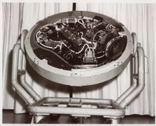
aerial film (Kodak type 3400 film), with base thickness 2,5 mil (6,35 μm) (Burnett, 1982). This thin base film enabled a several thousand feet long film to carry, expose and return. The ARGON system – unlike CORONA– was a pressurized envelope, and a vacuum platen kept the film absolutely flat during exposure, so there was no need for reseaus (Technical Explanation). The camera had no image motion compensation, so from the theoretical pixel size (150 meters) and from the approximate speed of the satellite (8000 m/sec) the exposure time could not exceed 18 msec (Figure 1).
Figure 1: The ARGON camera. This 3 inch focal length camera flying on CORONA satellites was the primary global mapping device of US Army Mapping Service in the first half of 1960’s.
https://www.nro.gov/Portals/65/images/CAL_Photo _45.jpg
1.4 ARGON Imagery in the Digital Era
Photos collected by a series of film-based reconnaissance satellites (KH ‘KeyHole’ series), in the 1960’s and 1970’s, including ARGON, CORONA, and LANYARD, has been declassified and made available in 1995, commonly referenced as Declassified Intelligence Satellite Photography (known as DISP) (McDonald, 1995). A digital archive of the imagery can be found on the EarthExplorer website (USGS EROS, 2010a), and ordered on-line through a shopping basket interface (USGS EROS, 2010b).
The systematic application of DISP imagery begun immediately after the declassification, and the high resolution CORONA imagery delivered its first results in 1998, enabling archaeologists to detect archaeological features in the arid regions of Asia Minor and the Middle East (Kennedy, 1998).
The ARGON imagery had much lower resolution,
but for compensation, it covers the -- from intelligence point of view uninterested -- remote environments, providing a unique opportunity for environmental reconstruction for the 1960s.
Bindschadler and Seider (1998) considered ARGON imagery as a precious resource for detecting the surface changes of Antarctic ice sheets in the 1960s, e.g., the margin changes of ice streams. Individual geometric modelling of ARGON photographs for Antarctica has been carried out successfully using spatial resection (Sohn and Kim, 2000). Several blocks of ARGON photographs have been successfully orthorectified over Greenland by the self-calibration block bundle adjustment model (Zhou et al., 2002). In 2006 Ye et al., (2017) applied ARGON imagery for stereo viewing of Antarctica, Li et al., (2017) used ARGON imagery to estimate ice flow patterns since 1960’s, and Ye et al. (2017) used ARGON imagery for generating DEM to estimate the ice volume of Antarctica in the 1960s.
2. Data
2.1 ARGON Imagery
The declassified Intelligence satellite photography (DISP) is disseminated by the USGS EROS Data Center (USGS EROS,2010a.) DISP images are available choosing the search engine options:
‘Declassified Data’. ARGON imagery is stored in the firstly (1996) declassified dataset. The image designators of the three consecutive images, used in this research are DS09034A038MC042_a, DS09034A038MC043_a and DS09034A038- MC044_a respectively. ‘DS’ stands for
’Declassified Satellite’ (imagery). The designator contains the mission number (9034A) the orbit (038) and the frame numbers (42, 43 and 44). The
‘MC’ abbreviation stands for ‘Mapping Camera’.
The images were acquired during the first successful ARGON mission (9034A). beginning 15th of May, 1962, and lasting for 4 days. The mission’s cover name was ‘Discoverer 41’, its COSPAR ID is 1962- 018A, and its Harvard designation is: ‘1962 Sigma 1’.
The satellite was launched from Vandenberg AFB, California, and the booster was the (at that time available) Thor-Agena configuration. The orbit had a 82,3 degree inclination, 284 km perigee, 632 km apogee and a 93.75 minutes period (Figure 2).
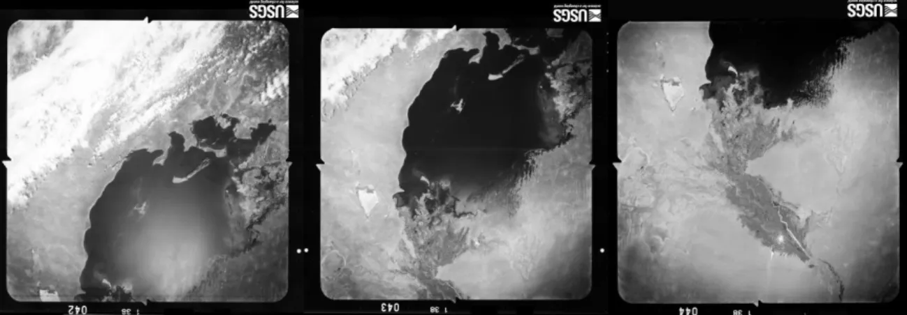
The scenes have a 60% overlap, scene Nr. 42 is 30%
cloudy, scene Nr. 43 is 10% cloudy and scene Nr.
44 is practically cloud-free. The ARGON photography has a film resolution of 30 line- pair/mm. This resolution equals to 33μm/line-pair.
Figure 2: The Scene Nr. 42, Nr. 43, and Nr. 44 of the ARGON mission Nr. 9034A, taken consecutively with 60 % overlap on orbit Nr. 38. (Scenes are 180° rotated) Source: USGS EROS Data Center
Table1: The size and resolution of digital ARGON images
Database identifier Size
(width × height) Resolution (dpi) Nr. 42. DS09034A038MC042_a 18093 × 18788 3649 Nr. 43. DS09034A038MC043_a 18404 × 19488 3649 Nr. 44. DS09034A038MC044_a 17366 × 18524 3629
The theoretical ground resolution is 140 meters, so the scanning of the film with 3628 dpi, resulted an approximately 30 meters pixel size, that is an oversampling of the original data, ensuring that no information loss due to the scanning of the image frames. To avoid confusion, the pixel resolution is referred to as 30 m in this paper unless stated otherwise.
2.2 Digital Elevation Model
The SRTM 1 Arc-Second Global Elevation dataset was used for multiple purposes in this research project. The applied elevation model dataset was merged of 1°×1° tiles, downloadable from USGS EROS Data Center. The extent of the elevation dataset is 55°-66° East and 39°-49° North. The primary use of the elevation dataset was supporting elevation data for Ground Control Points and orthorectification. Additionally the elevation dataset was used for GCP identification. For this
‘Roughness’ parameter image was calculated for the whole elevation dataset, and on this ‘Roughness’
image small and shallow water bodies were easily identifiable.
2.3. Ground Control Points
The Ground Control Points for ARGON scenes were collected in QGIS software. As a uniform and geometrically stable base for GCPs, both the SRTM DEM and the Google Satellite Imagery layer were applied as reference. For images Nr. 42, Nr. 43 and
Nr. 44, 36, 147 and 34 GCPs were collected respectively. Using the SRTM DEM elevation data, height coordinate was added to each GCP, and GCPs’ horizontal coordinates were stored in WGS84 latitude-longitude format. As the nominal pixel size of the ARGON imagery is 140 meters, and the scenes are panchromatic images, mostly large water body shorelines or shallow, small, temporal ponds’ centres provided the intensity contrast necessary to identify a feature on the image (Table 1).
3. Methods
In this chapter the geometrical modelling and the processing steps for orthocorrection of ARGON images are summarized.
3.1 Collinearity Equations
The relationship between the object space (ground) coordinates (Xgr,Ygr,Zgr) and image space (film) coordinates (ξ,η) is described by the collinearity equations of projective geometry.
𝜉𝑖𝑚𝑔= 𝜉𝑝− 𝑓𝑟11(𝑋𝑔𝑟− 𝑋0) + 𝑟12(𝑌𝑔𝑟− 𝑌0) + 𝑟13(𝑍𝑔𝑟− 𝑍0) 𝑟31(𝑋𝑔𝑟− 𝑋0) + 𝑟32(𝑌𝑔𝑟− 𝑌0) + 𝑟33(𝑍𝑔𝑟− 𝑍0) Equation 1
𝜂𝑖𝑚𝑔= 𝜂𝑝− 𝑓𝑟21(𝑋𝑔𝑟− 𝑋0) + 𝑟22(𝑌𝑔𝑟− 𝑌0) + 𝑟23(𝑍𝑔𝑟− 𝑍0) 𝑟31(𝑋𝑔𝑟− 𝑋0) + 𝑟32(𝑌𝑔𝑟− 𝑌0) + 𝑟33(𝑍𝑔𝑟− 𝑍0) Equation 2
where:
𝜉𝑖𝑚𝑔, 𝜂𝑖𝑚𝑔 are image space (film) coordinates,𝑋𝑔𝑟, 𝑌𝑔𝑟, 𝑍𝑔𝑟 are object space (local, ground) coordinates, 𝜉𝑝, 𝜂𝑝, 𝑓 are image principal point coordinates and focal length, 𝑋0, 𝑌0, 𝑍0 are satellite (camera) coordinates and 𝑟11, 𝑟12, … 𝑟33 are 3×3 rotation matrix elements, calculated from the 𝜔, 𝜑, 𝜅 camera attitude angles.
3.2 Object Space Local Cartesian Coordinate System
As in collinearity equations, the object space coordinates are in Cartesian coordinates, the GCPs’
ellipsoidal coordinates and levelled heights above sea level should be transformed into a local (topo- centered) Cartesian system. For this, GCPs’
ellipsoid coordinates and height (Φ, Λ, and h) are transformed to geocentric Cartesian coordinates:
𝑋 = (𝑁(𝛷) + ℎ)𝑐𝑜𝑠𝛷𝑐𝑜𝑠𝛬
Equation 3
𝑌 = (𝑁(𝛷) + ℎ)𝑐𝑜𝑠𝛷𝑠𝑖𝑛𝛬
Equation 4
𝑍 = [𝑁(𝛷) ∗ (1 − 𝑒2) + ℎ]𝑠𝑖𝑛𝛷
Equation 5
where 𝑁(Φ) is the radius of curvature in prime vertical, and e is the eccentricity of the WGS84 ellipsoid. As in the region around Aral Sea, the mean sea level (geoid) is below the surface of the Earth centred WGS84 ellipsoid (ERTF89 datum) with approximately 30 meters, 30 meter should be subtracted from height values derived from the SRTM DEM. (The spatial variance of the geoid height is only some meters, and this does not affect significantly the results. These geocentric coordinates are then transformed to local Cartesian coordinates, choosing Φ𝑐= 44°15′ and Λ𝑐 = 59°30′ as projection centre. In the first step Φ𝑐 and Λ𝑐 and h=0 values were substituted into Equation 3- 5., and Cartesian coordinates of 𝑋𝑐, 𝑌𝑐, 𝑍𝑐 projection centre coordinates are calculated. For each GCP, the local Cartesian (ground) coordinates are calculated:
[ 𝑋𝑔𝑟
𝑌𝑔𝑟 𝑍𝑔𝑟
] = [
−𝑠𝑖𝑛𝛬𝑐 𝑐𝑜𝑠𝛬𝑐 0
−𝑠𝑖𝑛𝛷𝑐𝑐𝑜𝑠𝛬𝑐 −𝑠𝑖𝑛𝛷𝑐𝑠𝑖𝑛𝛬𝑐 𝑐𝑜𝑠𝛷𝑐 𝑐𝑜𝑠𝛷𝑐𝑐𝑜𝑠𝛬𝑐 𝑐𝑜𝑠𝛷𝑐𝑠𝑖𝑛𝛬𝑐 𝑠𝑖𝑛𝛷𝑐
] ∙ [ 𝑋 − 𝑋𝑐
𝑌 − 𝑌𝑐 𝑍 − 𝑍𝑐
]
Equation 6
In the opposite way, first, local Cartesian (ground) coordinates are transformed into geocentric coordinates, and then ellipsoid coordinates are calculated using:
𝛷 = 𝑎𝑟𝑐𝑡𝑎𝑛 (𝑍 + 𝑒′2∙ 𝑏 ∙ 𝑠𝑖𝑛3𝛩 𝑝 − 𝑒′2∙ 𝑎 ∙ 𝑐𝑜𝑠3𝛩)
Equation 7 𝛬 = 𝑎𝑟𝑐𝑡𝑎𝑛 (𝑌
𝑋)
Equation 8 ℎ = 𝑝
𝑐𝑜𝑠𝛩− 𝑁(𝛷)
Equation 9 where a and b are the semi-major and semi-minor axes of WGS84 ellipsoid, 𝑁(Φ) is the curvature radius in prime vertical, 𝑝 = √𝑋2+ 𝑌2 , Θ = 𝑎𝑟𝑐𝑡𝑎𝑛 (𝑍∙𝑎
𝑝∙𝑏) and 𝑒′2=𝑎2−𝑏2
𝑏2 (Bowring, 1967).
3.3 Interior Orientation Parameters
This section focuses on the transformation between the digital image coordinate system (x,y) and the film (camera) coordinates (ξ,η) defined by the fiducial points. Ye et al., (2017) used a quadratic polynomial transformation between digital image and film coordinates. The application of this very precise transformation (eliminating also most of the interior deformations of the film and the scanning inaccuracies) however requires a Camera Calibration report, that contains the actual (not only the intended) coordinates of the fiducial points. In the absence of the Camera Calibration report, a rigid, 2D-Helmert transformation was applied on image coordinates (x,y) to obtain film (camera) coordinates (ξ,η):
[𝜉
𝜂] = [𝛿𝜉 ∙ 𝑐𝑜𝑠𝛼 𝛿𝜂 ∙ 𝑠𝑖𝑛𝛼
−𝛿𝜉 ∙ 𝑠𝑖𝑛𝛼 𝛿𝜂 ∙ 𝑐𝑜𝑠𝛼] ∙ [𝑥 − 𝑥𝑐 𝑦 − 𝑦𝑐]
Equation 10
where α is the angle between the digital image coordinate system and film (camera) coordinate system originating mostly from improper scanning.
δ𝜉 and δ𝜂 are pixel sizes in mm, 𝑥𝑐 and 𝑦𝑐 are digital image center coordinates. The film (camera) coordinates of the FMs’ was estimated in this way:
the difference of digital image coordinates of neighbouring FMs multiplied by digital image resolution resulted, that FMs were placed around 2cm distance from each other. As FMs form a quadrangular fence around image content, using this characteristic distance, the film (camera) coordinates of FMs are simply multiples of 2cm.
A least squares adjustment to estimate the five coefficients of the transformation (in Equation 10) were calculated for each image, using FM image and film coordinates. The result of adjustment provided the five unknown. Substituting these values into Equation 10, and calculating the residuals resulted, that FMs’ locations on film are
not exactly at the same coordinate as supposed, so during manufacturing the FMs were not placed with proper precision. Missing the Camera Calibration report, the exact (measured) location of FMs’ is not known, but as measured on the digital image, this discrepancy was found to be 5-10(!) pixels.
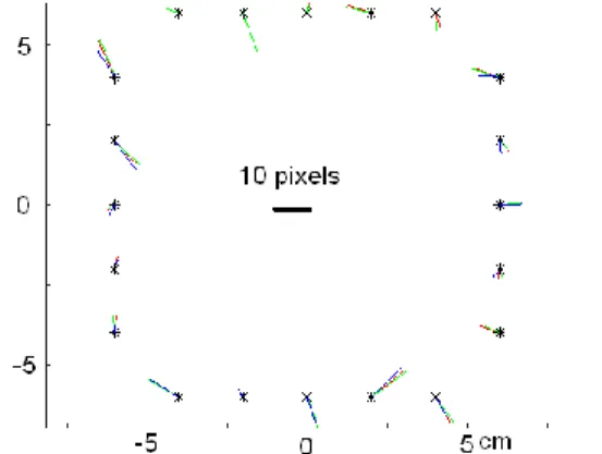
Repeating this calculation for each 3 ARGON images, the residual errors for each FM were calculated and showed on Figure 3.
Figure 1: Residual errors of the coordinates of fiducial marks for three ARGON images. As residual errors of the fiducial marks for each 3 images are similar, the source of error is the improper manufacturing of the camera, not any nonlinear deformation of the film
It is clearly seen, that these residuals are very similar for each image, so their origin is not a stochastic process as nonlinear film deformation or scanning error, but the inaccurate positioning of the FMs. For any FM, the three residuals show very strong correlation, and the RMS error of residuals is 1.61 and 0.63 pixels (in x and y directions). This also indicates that the deformation originating from nonlinear film deformations or scanning problems are in this magnitude. For each image, the coefficients for the reverse transformation (from film coordinates to digital image coordinates) were also calculated using the adjacent five coefficients, ensuring, that applying the forward and reverse transformation in succession, the twice transformed coordinates should equal to the original coordinates.
3.4 Space Resection
Space resection is the method used for calculating the satellite (camera) position and attitude using GCPs. If one could know the six exterior orientation (EO) parameters for an ARGON image, for any point (represented by their ground coordinates) its’
digital image coordinates could be calculated using first Equation 1 and Equation 2 to get film coordinates, and in a second step using the reverse of Equation 10 to get image coordinates. This would
be true for any GCP, collected for the respective image. We could formulate this as:
𝑥𝑖𝑐𝑎𝑙𝑐= 𝑓𝑥(𝑋𝑔𝑟,𝑖, 𝑌𝑔𝑟,𝑖, 𝑍𝑔𝑟,𝑖, 𝑋0, 𝑌0, 𝑍0, 𝜔, 𝜑, 𝜅) Equation 11
𝑦𝑖𝑐𝑎𝑙𝑐= 𝑓𝑦(𝑋𝑔𝑟,𝑖, 𝑌𝑔𝑟,𝑖, 𝑍𝑔𝑟,𝑖, 𝑋0, 𝑌0, 𝑍0, 𝜔, 𝜑, 𝜅) Equation 12
where 𝑥𝑖𝑐𝑎𝑙𝑐 and 𝑦𝑖𝑐𝑎𝑙𝑐 are the calculated image coordinates, i index represents the i-th GCP, and the meaning of EO parameters is discussed in Chapter 3.1. As measurements are erroneous, the digital image coordinates calculated from ground coordinates of the respective GCP would not exactly equal to the coordinates read out from the digital image and stored for the same GCP, however these values would be quite close to them. Least squares theorem states, that if in Equation 11 and in Equation 12. not the proper (‘true’) EO parameters would have been used, the absolute value of the differences between the calculated and measured image coordinates would be grater, than in the case of ‘true’ parameters. So this could be rewritten as a condition: in the case of applying the proper values of EO parameters in Equations 11 and 12, the sum of the squares of the differences of the measured and calculated coordinates should be minimal.
Formally:
∑ {[𝑥𝑖𝑚𝑒𝑎𝑠− 𝑓𝑥(𝑋𝑔𝑟,𝑖, 𝑌𝑔𝑟,𝑖, 𝑍𝑔𝑟,𝑖, 𝑋0, 𝑌0, 𝑍0, 𝜔, 𝜑, 𝜅)]2+ [𝑦𝑖𝑚𝑒𝑎𝑠− 𝑓𝑦(𝑋𝑔𝑟,𝑖, 𝑌𝑔𝑟,𝑖, 𝑍𝑔𝑟,𝑖, 𝑋0, 𝑌0, 𝑍0, 𝜔, 𝜑, 𝜅)]2 }
𝑁𝑟.𝑜𝑓 𝐺𝐶𝑃𝑠
𝑖=1
≔ 𝑚𝑖𝑛
(𝑋0, 𝑌0, 𝑍0, 𝜔, 𝜑, 𝜅)
Equation 13
This minimal condition fulfils, if all six partial derivatives of the left hand side of Equation 13 equal zero. This leads to six algebraic equations that can be solved using matrix algebra. As equations are not linear function of the EO parameters, an iterative process is required. For this we need the initial values of the parameters. As images were taken with almost vertical camera axis, for camera horizontal coordinate estimation the average of GCPs X and Y coordinates can be used, and Z can be chosen as nominal satellite orbit height above Earth’s surface. The almost vertical camera axis also means, that rotations along x and y axes are zeros (𝜔 = 𝜑 = 0), and only image azimuth angle should be estimated with some degree accuracy. The details of the calculation with proper theoretical background can be found in Sohn and Kim, 2000.
3.5 Camera Principal Point and Lens Distortion If the result of the space resection is not satisfactory, i.e. the residuals (the differences of the measured
and calculated image coordinates of the GCPs) are too large, it can be supposed, that other factors degrading image geometry cannot be neglected.
Some of these factors are the systematic errors of the frame camera. A very common problem, that the lens optical axis is not perpendicular to the film plane, and the optical axis does not point into the film centre point (defined by FMs). In this case, when applying the collinearity equations, (Equations 1 and 2.) the principal point coordinates cannot be supposed to be zero (𝜉𝑝≠ 0 and 𝜂𝑝≠ 0).
Another inherent problem of frame cameras is radial lens distortion. This is based on the lens design deficiency, and results, that image points would be displaced radially from the image center (McGlone, 2013). The distortion can be modeled and compensated by the following corrections:
∆𝜉𝑟𝑎𝑑𝑖𝑎𝑙 = 𝜉′∙ {𝐾0+ 𝑟2[𝐾1+ 𝑟2(𝐾2+ 𝑟2𝐾3)]}
Equation 14
∆𝜂𝑟𝑎𝑑𝑖𝑎𝑙 = 𝜂′∙ {𝐾0+ 𝑟2[𝐾1+ 𝑟2(𝐾2+ 𝑟2𝐾3)]}
Equation 15
where 𝜉′= 𝜉 − 𝜉0 and 𝜂′= 𝜂 − 𝜂0 and the radial distance from image principal point is. 𝑟 =
√𝜉′2+ 𝜂′2 . The other effect that cannot be neglected is the decentering distortion, which is in the other hand, primarily a function of the imperfect assembly of lens elements, not the actual design (Wolf, 1974). The equations describing the decentering lens distortion are:
𝛥𝜉𝑑𝑒𝑐𝑒𝑛𝑡𝑒𝑟𝑖𝑛𝑔 = 𝑃1(𝑟2+ 2𝜉′2) + 2𝑃2𝜉′𝜂′ Equation 16
𝛥𝜂𝑑𝑒𝑐𝑒𝑛𝑡𝑒𝑟𝑖𝑛𝑔= 2𝑃1𝜉′𝜂′+ 𝑃2(𝑟2+ 2𝜂′2) Equation 17
The principal point coordinates and coefficient in Equations 14-17, namely: 𝐾0, 𝐾1, 𝐾2, 𝐾3 and 𝑃1, 𝑃2
are calculated from calibration measurements made by the manufacturer of the camera and published in a Camera Calibration report. Hereinafter the camera principal point coordinates and lens distortion equation coefficients are referred as ‘Camera coefficients’.
3.6 Atmospheric Refraction
Atmospheric refraction correlates closely with the density of the atmosphere and can result in outward displacement in the image plane (Bertram, 1966).
As other authors reported a maximum displacement of 1/12th of pixel size (Zhou et al., 2002, Wang et al., 2016 and Ye et al., 2017) so it’s effect was neglected.
3.7 Modified Space Resection Algorithm
If it is obvious, that systematic errors caused by the camera imperfection should be considered in the ARGON image orthocorrection process, but Camera Calibration report is missing, applying the space resection method, besides the EO parameters, the camera parameters (principal point coordinates and lens distortion equation coefficients) can be also estimated. If one could know the – besides the six exterior orientation (EO) parameters the principal point and lens distortion parameters – for the j-th ARGON image, for any point (represented by their ground coordinates) its’ digital image coordinates could be calculated using first Equation 1 and Equation 2 to get film coordinates, and in a second step applying Equations 14-17 for correcting film coordinates and in third step using the reverse of Equation 10 to get image coordinates. This would be true for any GCP, collected for the respective image. We could formulate this as:
𝑥𝑖𝑐𝑎𝑙𝑐,(𝑗)= 𝑓𝑥(X𝑔𝑟,𝑖(𝑗), Y𝑔𝑟,𝑖(𝑗), Z𝑔𝑟,𝑖(𝑗), X0(𝑗), Y0(𝑗), Z0(𝑗), 𝜔(𝑗), 𝜑(𝑗), 𝜅(𝑗), 𝜉𝑝, 𝜂𝑝, 𝐾0, 𝐾1, 𝐾2, 𝐾3, 𝑃0, 𝑃1)
Equation 18
𝑦𝑖𝑐𝑎𝑙𝑐,(𝑗)= 𝑓𝑦(X𝑔𝑟,𝑖(𝑗), Y𝑔𝑟,𝑖(𝑗), Z𝑔𝑟,𝑖(𝑗), X0(𝑗), Y0(𝑗), Z0(𝑗), 𝜔(𝑗), 𝜑(𝑗), 𝜅(𝑗), 𝜉𝑝, 𝜂𝑝, 𝐾0, 𝐾1, 𝐾2, 𝐾3, 𝑃0, 𝑃1)
Equation 19
where 𝑥𝑖𝑐𝑎𝑙𝑐,(𝑗) and 𝑦𝑖𝑐𝑎𝑙𝑐,(𝑗) are the calculated image coordinates, i index represents the i-th GCP, j is the index of the j-th image, the meaning of EO parameters is discussed in Chapter 4.1. The 𝜉𝑝 and 𝜂𝑝 principal point coordinates and 𝐾0, 𝐾1, 𝐾2, 𝐾3, 𝑃0, 𝑃1 lens distortion coefficients are discussed in Chapter 4.5. Analysing the result of the least squares estimation, it could be seen, that especially the radial lens distortion parameters highly correlate with the satellite height parameter, so they cannot be estimated independently. The mean difference of these two parameters, that satellite height is unique to each ARGON image, while lens distortion parameters are the same for all images (taken by the same camera). To overcome this problem a modified space resection algorithm should be applied, where more than one ARGON images are used. In this modified space resection algorithm, the condition to be fulfilled is the same:
the sum of the squares of the difference of the measured and the calculated image coordinates of the GCPs should be minimal. The difference from the simple space resection method, is that, besides the EO parameters, the calculated film coordinates are the function of image principal point coordinates, and additionally on these film coordinates are lens correction applied.
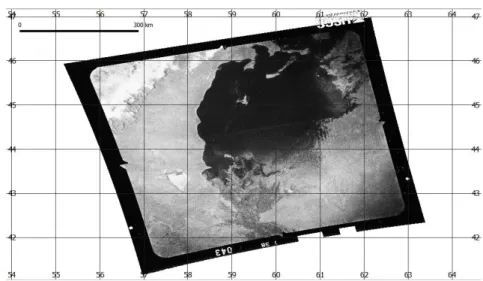
Figure 4: Orthocorrected ARGON image Nr. 43. Earth’s curvature is responsible for the elongation of image edges, and the apparent shearing is caused by the native projection (equidistant cylindrical) of the orthocorrected image
On the left hand side of the Equation 20, the double summation means, that the minimal condition should be fulfilled for all three images, for all GCPs respectively. On the right hand side we see, that the minimum is the function of 26 variables: 3×6+8 where the number of images (3) should be multiplied by the number of EO parameters (6) plus the principal point coordinates (2) and lens distortion correction coefficients (6).
∑ ∑ {[𝑥𝑖𝑚𝑒𝑎𝑠,(𝑗)− 𝑓𝑥(𝑋𝑔𝑟,𝑖(𝑗), 𝑌𝑔𝑟,𝑖(𝑗), 𝑍𝑔𝑟,𝑖(𝑗), 𝑋0(𝑗), 𝑌0(𝑗), 𝑍0(𝑗), 𝜔(𝑗), 𝜑(𝑗), 𝜅(𝑗), 𝜉𝑝, 𝜂𝑝, 𝐾0, 𝐾1, 𝐾2, 𝐾3, 𝑃0, 𝑃1)]2+ [𝑦𝑖𝑚𝑒𝑎𝑠,(𝑗)− 𝑓𝑦(𝑋𝑔𝑟,𝑖(𝑗), 𝑌𝑔𝑟,𝑖(𝑗), 𝑍𝑔𝑟,𝑖(𝑗), 𝑋0(𝑗), 𝑌0(𝑗), 𝑍0(𝑗), 𝜔(𝑗), 𝜑(𝑗), 𝜅(𝑗), 𝜉𝑝, 𝜂𝑝, 𝐾0, 𝐾1, 𝐾2, 𝐾3, 𝑃0, 𝑃1)]2
}
𝑁𝑟.𝑜𝑓 𝐺𝐶𝑃𝑠 𝑜𝑓 𝑖𝑚𝑎𝑔𝑒 𝑗
𝑖=1 𝑁𝑟.𝑜𝑓 𝑖𝑚𝑎𝑔𝑒𝑠
𝑗=1
≔ 𝑚𝑖𝑛
(3𝑥[𝑋0(𝑗), 𝑌0(𝑗), 𝑍0(𝑗), 𝜔(𝑗), 𝜑(𝑗), 𝜅(𝑗)], 𝜉𝑝, 𝜂𝑝, 𝐾0, 𝐾1, 𝐾2, 𝐾3, 𝑃0, 𝑃1)
Equation 20
4. Results
The primary result of the processing chain is the set of exterior orientations (EO) for each image and the camera coefficients, obtained using the modified space resection algorithm (Chapter 3.7). For orthoimage production simulated GCPs were generated for each ARGON image, and Rational Polynomial Camera model coefficients were calculated (Grodeczki, 2001). For image Nr. 43 the generated orthoimage can be seen on Figure 4.
5. Discussion
Ye et al., (2017) published a table that summarises the previous work of other authors for orthocorrection of ARGON imagery. The table lists the applied corrections and its effect on RMS error of residuals. Space resection methods based on GCPs without camera calibration yielded generally 150-200 meter RMS errors, and application of camera calibration coefficients (either estimated, or readout from Camera Calibration report) reduced RMS error to 100-120 meters. This work presented here is in good agreement with these results. The
RMS error of ARGON image Nr. 43, applying a space resection method were 3.27 pixels in x, and 2.94 pixels in y direction. Considering camera coefficients and applying a modified space resection algorithm, the respective RMS errors are 2,89 pixel in x and 2.65 pixels in y direction. As the pixel size of the digital image is 30 meters, the RMS errors in each direction are below 100 meter. Using the relatively great number (144) of GCPs for image Nr.
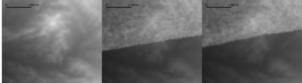
43, the image was also corrected by a 3rd order polynomial transformation. However RMS errors of GCPs are similar for both methods, the orthocorrection method seems more favourable, as the method successfully eliminates the effect of relief displacement, causing an almost 200 meter shrinking of the image edge due to the hilly terrain (see Figure 5b and 5c.).
Acknowledgement
The author expresses sincere appreciation to the European Union's project DSinGIS-Doctoral Studies in Geoinformation Sciences №585718-EPP- 1-2017-1-HU-EPPKA2-CBHE-JP (2017-3069/001).
Figure 5: a, Detail of the SRTM Elevation model representing surface heights on the Southern edge of the orthocorrected ARGON image Nr. 43. b, ARGON image Nr. 43, rectified by 3rd order polynomial transformation. c, ARGON image Nr. 43, orthocorrected by the presented method. However RMS error of the GCPs were similar for both methods, in the case of orthocorrection, the relief displacement is also corrected, causing an almost 200 meter shift of the image edge at hilly terrain.
References
Bertram, S., 1966, Atmospheric Refraction.
Photogrammetric Engineering, Vol. 32, 76-84.
Bindschadler, R. and Vornberger, P., 1998, Changes in the West Antarctic Ice Sheet Since 1963 from Declassified Satellite Photography, Science, Vol.
279, 689-692.
Bowring, B., 1976, Transformation from Spatial to Geographical Coordinates. Survey Review, Vol.
23, 323-327.
Burnett, M. G., 1982, Hexagon (KH-9) Mapping Camera Program and Evolution. (Director of Special Projects, Office of the Secretary of the Air Force).
Grodecki, J., 2001, IKONOS Stereo Feature Extraction-RPC Approach. Proceedings of ASPRS 2001 Conference, St. Louis, April 23-27.
Kennedy, D., 1998, Declassified Satellite Photographs and Archaeology in the Middle East: Case Studies from Turkey. Antiquity, Vol.
72, 553-561.
Li, R., Ye, W., Qiao, G., Tong, X., Liu, S., Kong, F.
and Ma, X., 2017, A New Analytical Method for Estimating Antarctic Ice Flow in the 1960s from Historical Optical Satellite Imagery. IEEE Transactions on Geoscience and Remote Sensing, Vol. 55, 2771-2785.
McDonald, R. A., 1995, CORONA: Success for Space Reconnaissance, A Look into the Cold War and a Revolution In Intelligence.
Photogrammetric Engineering and Remote Sensing, Vol. 61, 689-720.
McGlone, J. C., 2013, Manual of Photogrammetry, 6th edition, (Bethesda, Maryland: American Society for Photogrammetry and Remote Sensing).
Sohn, H., G. and Kim, K. T., 2000, Horizontal Positional Accuracy Assessment of Historical ARGON Satellite Photography. KSCE Journal of Civil Engineering, Vol. 4, 59-65.
Technical Explanation of Project ARGON, https://www.nro.gov/Portals/65/documents/foia/
CAL-Records/Cabinet3/DrawerC/3%20C%200- 011.pdf
USGS EROS, 2010a, EarthExplorer, URL:
https://earthexplorer.usgs.gov/ US geological Survey, Earth Resources Observation and Science (last date accessed: 01. September 2020).
USGS EROS, 2010b, USGS EROS Archive - Declassified Data - Declassified Satellite Imagery - 1, URL: https://doi.org/10.5066/- F78P5XZM, US Geological Survey, Earth Resources Observation and Science (last date accessed: 01. September 2020).
Wang, S., Liu, H., Yu, B., Zhou G. and Cheng, X., 2016, Revealing the Early Ice Flow Patterns with Historical Declassified Intelligence Satellite Photographs Back to 1960s. Geophysical Research Letters, Vol. 43, 5758-5767.
Wolf, P. R., 1974, Elements of Photogrammetry, 1st edition, (McGraw-Hill)
Ye, W., Qiao, G., Kong, F., Ma, X., Tong, X. and Li, R., 2017, Improved Geometric Modeling of 1960s KH-5 ARGON Satellite Images for Regional Antarctica Applications.
Photogrammetric Engineering and Remote Sensing, Vol. 83, 477-491.
Zhou, G., Jezek, K., Wright, W. Rand, J., and Granger, J., 2002, Orthorectification of 1960s Satellite Photographs Covering Greenland. IEEE Transactions on Geoscience and Remote Sensing, Vol. 40, 1247-1259.