On the calculation of the surface entropy in computer simulation

On the calculation of the surface entropy in computer simulation

Marcello Sega,

George Horvai,

and Pál Jedlovszky,

1

Faculty of Physics, University of Vienna, Boltzmanngasse 5, A-1090 Vienna, Austria

2

Department of Inorganic and Analytical Chemistry, Budapest University of Technology and Economics, Szt. Gellért tér 4, H-1111 Budapest, Hungary

3

Department of Chemistry, Eszterházy Károly University, Leányka utca 6, H- 3300 Eger, Hungary

Running title: Calculation of the Surface Entropy

*Electronic mail: marcello.sega@univie.ac.at (MS), jedlovszky.pal@uni-eszterhazy.hu (PJ)

Abstract

The surface excess of the entropy at the liquid-vapour interface of argon and water are calculated in a broad temperature range in three different ways involving the computer simulation determination of the surface tension. The three methods include (i) the calculation of the analytical derivative of a suitably chosen function fitted to the surface tension vs.

temperature data, (ii) calculation of the numerical derivative of these data, and (iii) direct determination of the surface entropy through the surface excess of the energy. Our results show that this latter method provides inaccurate results with large error bars, and the calculation of the surface entropy this way with reasonable accuracy would require unfeasibly long simulations. On the other hand, the use of the numerical and the analytical derivatives leads to compatible results that can be obtained in a computationally feasible way in both cases. Thus, the present results suggest that the surface entropy, determined as the derivative of the surface tension vs. temperature data, can be used to calculate the surface excess of the energy in a computationally efficient way.

Keywords: Surface entropy; surface tension; computer simulation, liquid-vapour interface

1. Introduction

Surface tension is a thermodynamic quantity of key importance when studying interfacial systems either experimentally, or by computer simulation methods. By definition, the surface tension, , is the reversible work needed to the creation of a unit area of surface at constant temperature (T), volume (V), and number of particles (N) of all types. In other words, it is the derivative of the Helmholtz free energy (F) with respect to its extensive counterpart, i.e., surface area (A) [!1]:

T V

A N

F

, ,



 







 

 . (1)

Surface tension can be routinely calculated in computer simulations either through the mechanical route, using the relation [!1]

^{ }

 



where pN and pL are the normal and lateral components of the pressure tensor, respectively, and z stands for the position along the interface normal axis, or through the thermodynamic route using eq. 1 [!2]. It should be noted that in computer simulations, instead of the full pressure tensor, often only its virial contribution is used in eq. 2; however, this treatment might lead to a systematic error in the computed surface tension value due to the neglect of its ideal gas contribution [!3].

The temperature derivative of the surface tension, often associated with (minus) the surface entropy [!4], can also be of great importance in certain cases, e.g., when the temperature (and hence also the surface tension) along the surface is non-uniform, resulting in

the Bénard-Marangoni convection [!5]. The two surface tension anomalies of liquid water are also related to this derivative [!6], as it goes through a maximum at 277 K [!7,8], and through a minimum at 530 K [!9] rather than decreasing monotonously with increasing temperature, as in other molecular liquids. These anomalies are related to the formation of an infinite H- bonding network of the water molecules, as similar behaviour was observed for network forming polymers [!10], and can be explained by a two-state mixture model (at 277 K) [!11], and by the percolation transition of the two-dimensional network of the surface molecules (at 530 K) [!12,13].

The surface entropy can be calculated from a set of computer simulations done at different temperatures by performing the derivation of the  vs. T data. Alternatively, several direct methods, involving simulations only at the temperature of interest, have been proposed in the literature [!4,14,15]. In this paper, we compare the accuracy of several such methods, using the analytical derivative of an appropriate function fitted to the surface tension vs.

temperature data, as a reference. The methods that we test here are chosen because of their computational simplicity. Performing a meaningful comparison of such methods has been made possible by (i) the continuous development of the routinely available computing power, which now enables one to accurately calculate the surface tension within reasonable time, and (ii) the existence of a suitable functional form that can be used to fit the surface tension vs.

temperature data with very high accuracy for markedly different systems. Here we use two test systems, and apply the chosen methods to the liquid-vapour interface of argon as well as of water. The paper is organized as follows. The main points of the theory of the surface excess quantities and of the method considered are described in sec. 2. Details of the simulations performed are given in sec. 3. Finally, the obtained results are presented and discussed in sec. 4.

2. Theory

2.1. Surface excess and the Gibbs dividing surface

The surface excess of any extensive thermodynamic quantity, X, can be defined as [!1]

β β α α IF

s X x V x V

X    , (3)

where indices  and  refer to the corresponding coexisting bulk phases, s stands for the surface excess, IF denotes the interfacial system, V is for the volume, and x denotes the density of the extensive quantity X in the corresponding bulk phase, i.e., x = X/V. The value of the surface excess, i.e., X^s depends, in general, on the particular choice of the position of the (infinitely thin) surface that divides the interfacial system to two coexisting phases. Using the particular choice for this surface, called the Gibbs dividing surface or the equimolar surface, that satisfies the equation

s 0



i i in

 , (4)

where i and n_i^s stand for the chemical potential and surface excess of the molar number of component i, respectively, has several advantages. Thus, in this case the surface tension, defined through eq. 1, can be associated with the surface excess of the Helmholtz free energy,

Fs [!1], and hence its temperature derivative,

s ,

, s ,

,

T S F

T NV A NV A



 















 



 









(5)

with the surface excess of the entropy, S^s, often referred to simply as the surface entropy.

Using the relation

T F S U

s

s  s  , (6)

where U is the internal energy, the calculation of S^srequires, besides the surface tension itself, only the surface excess of the internal energy, U^s according to eqs. 3 and 4.

In a one component system, eq. 4 simplifies to n^s = 0, which, using eq. 3 and considering a simulation box with the edge length of LZ along the interfacial normal axis, Z, can be written as





G β

αZ  L Z  L

    , (7)

where  is the number density, and ZG denotes the position of the Gibbs dividing surface along the axis Z. From eq. 7, the position of the Gibbs dividing surface can be derived as











 _{Z α}^IF ^β

G L

Z . (8)

2.2. Derivative of the surface tension vs. temperature data

Conceptually probably the simplest way of obtaining the surface entropy is using eq.

1, and calculating the derivative of the surface tension vs. temperature data. This can be done either by fitting an appropriate function to several (T) points, or, simply, by computing the derivative d/dT numerically, using a suitable finite difference scheme. The drawback of using the analytical derivative is that it requires simulations at several different temperatures to allow a meaningful fitting of the data. However, besides the particular choice of the functional form used in the fitting procedure, this method is free from additional approximations. On the other hand, the calculation of the numerical derivative is computationally less expensive, however, the accuracy of the result depends on the choice of

the temperature interval, which should be (i) small enough to provide a reasonable approximation of d/dT, and (ii) large enough to provide a much larger difference of the corresponding surface tension values than their statistical uncertainty.

Similarly to our previous paper [!16], here we also fit the  vs. T data by the function proposed by Vargaftik et al., i.e.,



 



 



 



 

 



 



 



c c

1 1

1 T

b T T

B T



 , (9)

since it accurately describes the experimental surface tension of water in a very broad range of temperatures [!17]. The fit uses four parameters, i.e., B, b, , and Tc, the latter being the critical temperature. The surface entropy can then be obtained from the derivative of eq. 9, i.e.,

c c c

s c 1

T/

- 1 d

d

T b T B T T T S T

 

 



 



 







 . (10)

To perform the numerical derivative, we used the first order forward and backward differences:

 

) ) (

( d

d O T

T T T T

T  







   

 (11)

and

 

d

d O T

T T T T

T  







  

 (12)

at the extremal temperatures, and the second order centred difference:

 

) 2 (

) (

d

d ₂

T T O

T T T T

T  











  

 (13)

for the remaining points.

2.3. Direct calculation through the surface energy

Considering that V^IF = ALZ, A being the cross-section area of the simulation box, and using eqs. 3 and 8, U^scan be written as

 















 

 

 







 ^β

β α

β IF α Z

β α

β IF IF Z

β β α α IF

s U u V u V U AL u AL 1 u

U  













   

























 

 ^{IF IF IF β} u ^{β IF} u^β

V

U , (14)

u^ and u^ being the energy densities in the corresponding bulk phases.

The determination of (/T) through eqs. 5, 6 and 14 requires thus (i) the values of UIFand F^s  , which can be easily obtained from the simulation of the interfacial system, and (ii) also those of u^, u^, ^ and ^, which can be taken from the energy and number density profiles along the interface normal axis, Z, as the constant values corresponding to the two bulk phases. Note that if periodic boundary conditions are applied, the excess internal energy and free energy obtained this way have to be divided by the number of interfaces present in the basic box (i.e., two in our case). Alternatively, u^ and u^ can also be easily determined from short simulations of the two bulk phases, done at the same temperature and density as those of the corresponding bulk parts of the interfacial system simulated, as the ratio of the total internal energy and the volume of the simulation box. Although this latter treatment, employed also here, requires two additional bulk phase simulations besides the interfacial one, it avoids the complication that arises when the total energy of the interfacial system needs to be distributed among the interaction sites in the calculation of the energy density profile, especially when certain contributions to the total energy are not pairwise additive (e.g., the reciprocal space contribution of the long range correction of the

electrostatic interaction when using Ewald summation [!18,19] or one of its particle mesh variants [!20,21]).

3. Molecular dynamics simulations

The liquid-vapour interface of argon as well as of water has been simulated on the canonical (N,V,T) ensemble, at six different temperatures each. In the case of argon, the basic simulation box, having the X, Y, and Z edge lengths of 40 Å, 40 Å, and 180 Å, respectively, has consisted of 2237 atoms, while in the case of water 1024 molecules have been placed in a 30 Å× 30 Å× 100 Å basic box (Z being the interface normal direction). The temperatures of the simulations have covered the range between 84.2 K and 114.3 K with a step of about 6 K (i.e., between 0.7 and 0.95 with a step of 0.05 in terms of reduced units) for argon, and the range between 300 K and 550 K with a step of 50 K for water. The temperature range considered here falls between the triple point and critical point of the system in both cases.

[!22]. Further, to evaluate u^ and u^ in eq. 14, the bulk liquid and vapour phase of both systems have also been simulated at the same temperatures as the interfacial systems. In these simulations, the basic box of the liquid and vapour phase has always contained 2048 and 21 argon atoms, or 649 and 20 water molecules, respectively. The edge lengths of the cubic basic box has always been chosen in such a way that the density of the bulk system has agreed with that of the corresponding bulk phase in the interfacial simulation; these values are collected in Tables 1 and 2 for argon and water, respectively.

Argon atoms have been described by the potential model of Rahman, which describes the interatomic interaction by a Lennard-Jones potential, having the distance and energy parameter values of  = 3.4 Å and (/kB) = 120 K (kB being the Boltzmann constant) [!23].

Water has been modelled by the rigid, non-polarizable, three-site SPC/E potential model

[!24]. In this model, the H atoms carry fractional charges of +0.4238e, compensated by the fractional charge of -0.8476e at the O atom. The O atom is also the centre of the Lennard- Jones interaction, corresponding to the distance and energy parameters of  = 3.166 Å and

 = 0.65 kJ/mol, respectively, while the O-H bond length and H-O-H bond angle are 1.0 Å

and 109.47^o, respectively [!24]. In the simulations, all interactions have been truncated to zero beyond the cut-off distance of 11 Å (in the case of water this refers to the distance of the O atoms). The long range part of both the electrostatic and dispersion interaction has been accounted for using the smooth Particle Mesh Ewald method [!21,25] with the grid spacing of 1.5 Å, and accuracy of the reciprocal space contribution of 10^-5 for the Coulomb and 10^-3 for the Lennard-Jones interaction. It should be noted that taking the long-range part of the Lennard-Jones interaction into account using an Ewald-based method is particularly important in the presence of an interface, as in this case the anisotropy of the system prevents the use of the analytical tail correction [!26]. The temperature of the systems has been controlled by the Nosé-Hoover thermostat [!27,28] with a relaxation time of 1 ps. The geometry of the water molecules has been kept rigid by means of the SETTLE algorithm [!29].

All simulations have been performed using the GROMACS 5.1 molecular dynamics program package [!30]. Equations of motion have been integrated in time steps of 1 fs. The systems have been equilibrated for 1 ns. Then, in the 5 ns long production stage of the simulations, the energy of the system and, in the case of the interfacial simulations, also the elements of the pressure tensor have been averaged over 5 ×10⁴ equilibrium sample configurations, separated by 0.1 ps long trajectories each. Finally, the surface tension of the interfacial systems has been calculated according to eq. 2.

4. Results and discussion

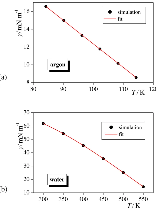
The surface tension values obtained for argon and water at the six-six temperatures considered are collected in Tables 1 and 2, respectively. Further, the (T) data corresponding to both systems are also plotted in Figure 1, along with their best fits with eq. 9. The parameters corresponding to the best fits are collected in Table 3. As is seen, eq. 9 provides an excellent fit of the simulated data in both cases. For this reason, we consider here the functions resulted from the analytical derivative of the fitted curves (eq. 10) as reference results, to which the data obtained by the other methods are compared.

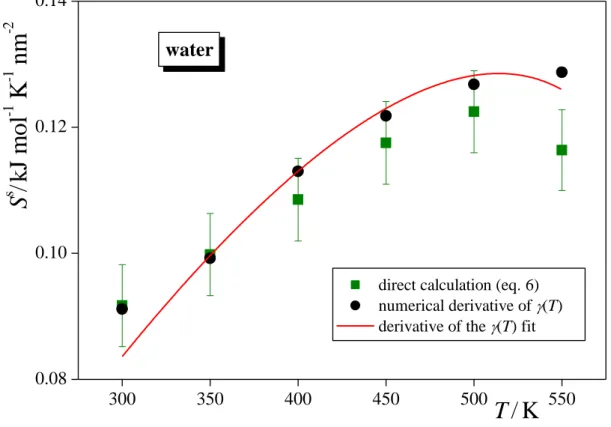
The numerical derivative of the (T) data along with the curves obtained from the analytical derivative of the fitted functions are shown in Figures 2 and 3 as obtained for argon and water, respectively. The surface entropy values obtained from the direct calculation are also included in these figures, while the energies of the two bulk and the interfacial system are collected in Tables 1 and 2 as obtained for argon and water, respectively. As is seen, the values corresponding to the numerical derivative agree well with the reference curve of eq. 10 in the entire temperature range considered for both systems. In most cases, the agreement is within error bars, and even if it is not, it usually does not exceed 2-3%. On the other hand, the data resulted from the direct calculation show a considerably worse agreement with the curves corresponding to the analytical derivative of the fitted (T) functions. More importantly, the error bars corresponding to these data are considerably, by one and, in several cases, even two orders of magnitude larger than those of the numerical derivatives. These surprisingly large error bars suggest that the data obtained by the direct calculation are very sensitive to the exact position of the equimolar surface, and small inaccuracies occurring in its determination are amplified when calculating the surface entropy. Considering that the position of the Gibbs dividing surface is determined through the densities of the coexisting bulk phases (see eq. 8),

accurate calculation of the surface entropy requires the determination of these densities with very high accuracy. These densities, however, have to be determined from the interfacial simulation (as they are already used as input data of the bulk ones), where (i) the Z ranges in which the two phases can be regarded as bulk ones, because all effects caused by the vicinity of the interface are vanished, and hence can be used to determine the bulk phase densities are not unambiguously defined, and (ii) the density profile even in the bulk-like parts of the system are affected by oscillations due to the capillary waves of the surface [!31]. Therefore, accurate enough determination of the bulk phase densities, and hence that of the surface entropy requires very long simulation of a very large interfacial system. This requirement makes the direct method, once hoped to be a computationally more efficient alternative of calculating the derivative of the  vs. T data, computationally rather inefficient. On the other hand, with the presently available computing capacities, d/dT can routinely be calculated using either the numerical derivative scheme (involving simulations at two or three temperatures), or that of the analytical derivative (involving 5-10 simulations), and these methods can provide compatible results with each other. It should finally be noted that the original purpose of developing the direct method was to provide access to the surface excess of the entropy through the surface excess of the energy [!14], our present results suggest that this relation (eq. 6) should rather be used in the other way around, namely that if the surface excess energy is needed to be calculated, it can computationally feasibly be done through the surface entropy, i.e., as

T T U^s

d d

 

 . (15)

Acknowledgement. This work has been supported by the Hungarian NKFIH Foundation under Project Nos. 119732 and 120075.

References

[1] J. S. Rowlinson, B. Widom, Molecular Theory of Capillarity, Dover Publications, Mineola, 2002, p. 11.

[2] G. J. Gloor, G. Jackson, F. J. Blas, E. de Miguel, J. Chem. Phys. 123 (2005) 134703.

[3] M. Sega, B. Fábián, P. Jedlovszky, J. Phys. Chem. Letters 8 (2017) 2608.

[4] Z. Q. Wang, D. Stroud, Phys. Rev. A 41 (1990) 4582.

[5] A. V. Getling, Rayleigh-Bénard Convection: Structures and Dynamics, World Scientific, Singapore, 1998.

[6] J. Pellicer, V. García-Morales, L. Guanter, M. J. Hernández, M. Dolz, Am. J. Phys. 70 (2002) 705.

[7] P. T. Hacker, Experimental Values of the Surface Tension of Supercooled Water, Technical note 2510, National Advisory Committee for Aeronautics, Washington D.

C., 1951.

[8] N. B. Vargaftik, B. N. Volkov, L. D. Voljak, J. Phys. Chem. Ref. Data 12 (1983) 817.

[9] IAPWS, Release on Surface Tension of Ordinary Water Substance. Available from:

http://www.iapws.org /relguide/surf.pdf, 1994.

[10] N. R. Bernardino, M. Telo da Gama, Phys. Rev. Letters 109 (2012) 116103.

[11] J. Hrubý, V. Holten, in: 14^th Int. Conf. Properties Water Steam, IAPWS, Kyoto, 2004, pp. 241-246.

[12] M. Sega, G. Horvai, P. Jedlovszky, Langmuir 30 (2014) 2969.

[13] M. Sega, G. Horvai, P. Jedlovszky, J. Chem. Phys. 141 (2014) 054707.

[14] K. S. Liu, J. Chem. Phys. 60 (1974)4226.

[15] E. Salomons, M. Mareschal, J. Phys: Condens. Matter 3 (1991) 3645.

[16] M. Sega, C. Dellago, J. Phys. Chem. B 121 (2017) 3798.

[17] N. B. Vargaftik, B. N. Volkov, L. D. Voljak, . Phys. Chem. Ref. Data 12 (1983) 817.

[18] P. Ewald, P. Ann. Phys 369 (1921) 253.

[19] S. W. de Leeuw, J. W. Perram, E. R. Smith, Proc. R. Soc. Lond. A 373 (1980) 27.

[20] T.; Darden, D.; York, L. Pedersen, J. Chem. Phys. 98 (1993) 10089.

[21] U. Essman, L. Perera, M. L. Berkowitz, T. Darden, H. Lee, L. G. Pedersen, J. Chem.

Phys. 103 (1995) 8577.

[22] M. Sega, B. Fábián, A. R. Imre, P. Jedlovszky, J. Phys. Chem. C 121 (2017) 12214.

[23] A. Rahman, Phys. Rev. 136 (1964) A405.

[24] H. J. C. Berendsen, J. R. Grigera, T. Straatsma, J. Phys. Chem. 91 (1987) 6269.

[25] C. L. Wennberg, T. Murtola, B. Hess, E. Lindahl, J. Chem. Theory Comput. 9 (2013) 3527.

[26] P. J. in’t Veld, A. E. Ismail, G. S. Grest, J. Chem. Phys. 127 (2007) 144711.

[27] S. A. Nosé, Mol. Phys. 52 (1984) 255.

[28] W. G. Hoover, Phys. Rev. A 31 (1985) 1695.

[29] S. Miyamoto, P.A. Kollman, J. Comp. Chem. 13 (1992) 952.

[30] S. Pronk, S. Páll, R. Schulz, P. Larsson, P. Bjelkmar, R. Apostolov, M. R. Shirts, J. C.

Smith, P. M. Kasson, D. van der Spoel, Bioinformatics 29 (2013) 845.

[31] S. Toxvaerd, J. Stecki, J. Chem. Phys. 102 (1995) 7163.

Tables

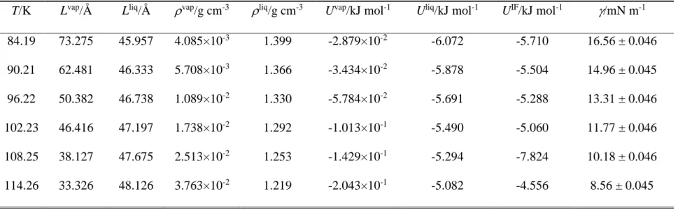
Table 1. Properties of the simulated systems of argon. L, N, and U stand for the basic box edge length, number of particles in the basic box, and energy of the system, respectively; superscripts vap, liq, and IF denote bulk vapour, bulk liquid, and interfacial simulations, respectively.

T/K L^vap/Å L^liq/Å ^vap/g cm^-3 ^liq/g cm^-3 U^vap/kJ mol^-1 U^liq/kJ mol^-1 U^IF/kJ mol^-1 /mN m^-1

84.19 73.275 45.957 4.085×10^-3 1.399 -2.879×10^-2 -6.072 -5.710 16.56 ± 0.046

90.21 62.481 46.333 5.708×10^-3 1.366 -3.434×10^-2 -5.878 -5.504 14.96 ± 0.045

96.22 50.382 46.738 1.089×10^-2 1.330 -5.784×10^-2 -5.691 -5.288 13.31 ± 0.046

102.23 46.416 47.197 1.738×10^-2 1.292 -1.013×10^-1 -5.490 -5.060 11.77 ± 0.046

108.25 38.127 47.675 2.513×10^-2 1.253 -1.429×10^-1 -5.294 -7.824 10.18 ± 0.046

114.26 33.326 48.126 3.763×10^-2 1.219 -2.043×10^-1 -5.082 -4.556 8.56 ± 0.045

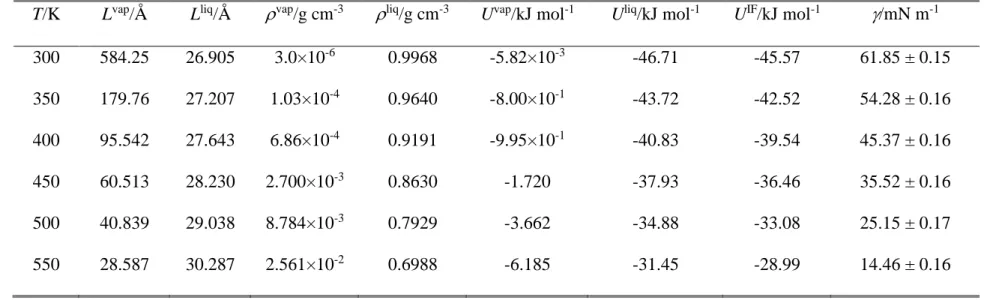
Table 2. Properties of the simulated systems of water. L, N, and U stand for the basic box edge length, number of particles in the basic box, and energy of the system, respectively; superscripts vap, liq, and IF denote bulk vapour, bulk liquid, and interfacial simulations, respectively.

T/K L^vap/Å L^liq/Å ^vap/g cm^-3 ^liq/g cm^-3 U^vap/kJ mol^-1 U^liq/kJ mol^-1 U^IF/kJ mol^-1 /mN m^-1

300 584.25 26.905 3.0×10^-6 0.9968 -5.82×10^-3 -46.71 -45.57 61.85 ± 0.15

350 179.76 27.207 1.03×10^-4 0.9640 -8.00×10^-1 -43.72 -42.52 54.28 ± 0.16

400 95.542 27.643 6.86×10^-4 0.9191 -9.95×10^-1 -40.83 -39.54 45.37 ± 0.16

450 60.513 28.230 2.700×10^-3 0.8630 -1.720 -37.93 -36.46 35.52 ± 0.16

500 40.839 29.038 8.784×10^-3 0.7929 -3.662 -34.88 -33.08 25.15 ± 0.17

550 28.587 30.287 2.561×10^-2 0.6988 -6.185 -31.45 -28.99 14.46 ± 0.16

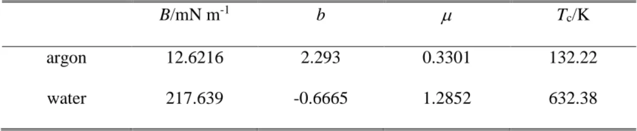
Table 3. Parameters obtained by fitting the simulated surface tension vs. temperature data of argon and water by eq. 9.

B/mN m^-1 b  Tc/K

argon 12.6216 2.293 0.3301 132.22

water 217.639 -0.6665 1.2852 632.38

Figure legend

Fig. 1. Surface tension of argon (top panel) and water (bottom panel) as obtained from our simulations at the six-six temperatures considered (full black circles), together with their fits according to eq. 9 (red solid curves). Error bars are always smaller than the symbols.

Fig. 2. Surface entropy of argon, as obtained from our simulations at the six temperatures considered through the calculation of the surface excess energy (eqs. 6 and 14, full green squares), from the numerical derivation of the surface tension vs. temperature data (full black circles), and from the analytical derivation of the function fitted to these data (red solid curve). Error bars are only shown when larger than the symbols.

Fig. 3. Surface entropy of water, as obtained from our simulations at the six temperatures considered through the calculation of the surface excess energy (eqs. 6 and 14, full green squares), from the numerical derivation of the surface tension vs. temperature data (full black circles), and from the analytical derivation of the function fitted to these data (red solid curve). Error bars are only shown when larger than the symbols.

Figure 1 Sega et al.

80 90 100 110 120

8 10 12 14 16

300 350 400 450 500 550

10 20 30 40 50 60 70

argon

 / m N m

T / K

simulation fit

water

simulation fit

T / K

 / m N m

(a)

(b)

Figure 2 Sega et al.

80 90 100 110 120

0.13 0.14 0.15 0.16 0.17 0.18

argon

S

/ k J m o l

K

n m

T / K

direct calculation (eq. 6) numerical derivative of (T) derivative of the (T) fit

Figure 3 Sega et al.

300 350 400 450 500 550

0.08 0.10 0.12 0.14

water

S

/ k J m o l

K

n m

T / K

direct calculation (eq. 6) numerical derivative of (T) derivative of the (T) fit

Figure 4.

Sega et al.

Table of Contents Graphics: