Academic Staff Performance Evaluation – Variants of Models

Academic Staff Performance Evaluation – Variants of Models

Jan Stoklasa, Jana Talašová, Pavel Holeček

Department of Mathematical Analysis and Applications of Mathematics, Faculty of Science, Palacký University

17. listopadu 1192/12, 771 46 Olomouc, Czech Republic

jan.stoklasa@upol.cz, talasova@inf.upol.cz, holecekp@inf.upol.cz

Abstract: In the paper we describe the development process of the academic staff performance evaluation model for Palacky University in Olomouc (Czech Republic).

Various alternatives of the mathematical solution are discussed. All the models share the same basic idea – we evaluate the staff member’s performance in the area of Pedagogical Activities and in the area of Research and Development. The input data for the models is obtained from structured forms containing information about all the activities performed by a current staff member in the respective year. We require an aggregated piece of information concerning the yearly performance of a particular staff member at a current work position (achievement of standard performance, achievement of excellence, etc.). In the first part of the paper we analyse a group of models that share the algorithm for normalized partial evaluations in both areas of interest (Pedagogical Activities, Research and Development); the partial evaluation normalization function is determined by the scores for standard and excellent performance (defined by the evaluator for different work positions and for both areas of interest separately). Models within this group differ by the aggregation operator used to calculate the overall performance evaluation – weighted arithmetic average (WA), OWA, and WOWA. The second part of the paper presents a model where partial evaluations are determined simply as multiples of standard score for the current work position and area of interest, but the aggregation of these partial evaluations is performed by a fuzzy-rule-based system. This fuzzy model is currently being implemented at Palacky University.

Keywords: evaluation; academic staff; aggregation; fuzzy model

1 Introduction

The general requirements on the model to be developed and used at Palacky University were as follows: It should a) include, if possible, every aspect of academic staff activity; b) use only easily verifiable and objective data; and c) be easy to work with. Other requirements were for the final evaluation: d) to

maximally reflect staff benefit to the Faculty; and e) not to be a simple average of partial evaluations in separate areas of activity, but to be able to appreciate excellent performance in any of the two evaluated areas (Pedagogical Activities - PA, Research and Development - RD).

The main objective of the model is to globally assess the performance and overall work load of each academic staff member in regular time intervals (annually). To achieve this, detailed information in a unified form concerning particular activities and outcomes of a particular academic staff member will be gathered. Aggregated overall evaluation information will also be available (at different levels of aggregation). As far as the aggregated evaluation is concerned, the desired output of the model was neither to arrange members of academic staff in order of their performance, nor to obtain crisp numerical evaluations interpretable only with difficulty. A rough piece of information concerning the performance of a particular academic staff member is sufficient for staff management. If more detailed information is needed, evaluations on lower levels of aggregation are available (i.e. multiples of standard score for each area of interest).

To be able to design a model with the desired properties, we studied general problems of quality assessment in high education institutions (see [1] for the Czech Republic and [2] for the EU), and fundamentals of human resource management (see [3]). At the same time we were looking for appropriate mathematical tools for these purposes (see [4, 5, 6, 7]). Various academic staff evaluation models currently used in the USA (see e.g. [8]), Canada ([9]), and Australia ([10, 11]) were subjected to a detailed analysis. Later, even the models recently designed at various Czech universities (see [12, 13, 14]) were analysed.

Models of performance assessment of whole departments were also studied (see [Babak Daneshvar Rouyendegh, Serpil Erol]) as well as business models of performance assessment (see [Lívia Róka-Madarász]). The analysis concentrated on both the contents and mathematical aspects of these evaluation models and resulted in the design of several academic staff evaluation models (see [15, 16]).

The models described later in the paper differ both in the manner of how members of academic staff are evaluated in separate areas of their activity and in the aggregation method for these partial evaluations (Weighted average, OWA, and WOWA operators were used; for the theory of aggregation operators see [5, 6];

we also considered fuzzy expert systems as a means of aggregation [17, 18]).

2 Preliminaries

The fundamentals of the fuzzy set theory (introduced in 1965 by Zadeh [19]) are described in detail, e.g., in [4]. Let U be a nonempty set (the universe). A fuzzy set A on U is defined by the mapping A U: 

 

0,1 . For each x U the value ( )A x

is called the membership degree of the element x in the fuzzy set A and A( ) is called the membership function of the fuzzy set A. The height of a fuzzy set A is the real number ^{hgt( )}A ^supx U_



A x^{( )}



. Other important concepts related to fuzzy sets are: a) the kernel of A, ^Ker

  

^{A  x U |A x( )1}



, b) the support of A,

 

Supp( )A  x U A x| ( )0 and c) the -cut of A, ^A^



^{x U A x | ( )}



, for

 

0,1

 .

A function ^{T: 0,1}

 

^2

 

^0,1 is called a triangular norm or t-norm if for all , , , [0,1]

    it satisfies the following four properties: 1) commutativity:

( , )   ( , ) 

T T , 2) associativity: T( , ( , )) T   T T( ( , ), )   , 3) monotonicity: if   ,   , then it holds that T( , )  T( , )  , and 4) boundary condition: T( ,1) .

A function ^{S: 0,1}

 

^2

 

^0,1 is called a triangular conorm or t-conorm if for all , , , [0,1]

    it satisfies the properties 1) - 3) from the previous definition and 4) the boundary condition: S( , 0) ^.

A function ^{N: 0,1}

   

^{ 0,1} satisfying conditions: a) N(0) = 1 and N(1) = 0, b) N is strictly decreasing, c) N is continuous and 4) N(N(x)) = x for all x

 

0,1 (N is involutive), is called a strong negation. For the purposes of this paper we consider the following strong negation: N x( ) 1 x, where ^x

 

^{0,1 .}

If T x y( , )N S N x N y( ( ( ), ( ))) for all x y, 

 

0,1 , we call S the N-dual t-conorm to T. Triangular norms and conoroms are used to define the intersection and union of fuzzy sets respectively. Let A and B be fuzzy sets on U. The intersection of A and B is a fuzzy set



A^T B



on U given by



A^T B



^{( )}x ^T A x B x( ( ), ( )) for all x U , where T is a t-norm. The union of A and B on U is a fuzzy set



A^S B



on U given by



A_SB



^{( )}x S A x B x( ( ), ( )) for all x U , where S is a t-conorm N- dual to T, for more details see [4]. Let A be a fuzzy set on U and B be a fuzzy set on V. Then the Cartesian product of A and B is a fuzzy set A_TB on U V given by (A_TB x y)( , )T A x B y( ( ), ( )) for all ( , )x y  U V. See [4] for more details on triangular norms and conorms. A binary fuzzy relation is any fuzzy set P on

U V .

In this paper we will use the product t-norm (T( , )    , for all , [0,1]) and the probabilistic sum t-conorm (S( , )        , for all  , [0,1]).

For the union, intersection and Cartesian product of fuzzy sets A and B based on

this t-norm and t-conorm we use the following notation:



^AB



^,



^AB



^and



^{A B}



respectively.

Let R denote the set of all real numbers. Fuzzy set C on R is called fuzzy number if it satisfies three conditions: 1) the kernel of C, Ker(C), is a nonempty set, 2) the-cuts of C, C_, are closed intervals for all  (0,1], and 3) the support of C, Supp(C), is bounded. The symbol F_N( )R denotes the family of all fuzzy numbers on R. If Supp( )C [ , ]a b , we call C a fuzzy number on the interval [a,b]. The family of all fuzzy numbers on the interval [a,b] will be denoted byF_N([ , ])a b .

Let A₁, A₂, ..., A_nF_N([ , ])a b , we say that A₁, A₂, ..., A_n form a fuzzy scale on [a,b]

if these fuzzy numbers form a Ruspini fuzzy partition (see [20, 21]) on [a,b] (i.e.

1 ( ) 1

 



iⁿ A xⁱ , for all x[ , ]a b ) and are numbered in accordance with their ordering.

The basics of linguistic fuzzy modelling were introduced by Zadeh in [22]. A linguistic variable is the quintuple (X, T(X), U, M, G) where X is the name of the linguistic variable, T(X) is the set of its linguistic values (linguistic terms), U is the universe, U[ , ]a b R, which the mathematical meanings (fuzzy numbers) of the linguistic terms are defined on, G is a syntactic rule (grammar) for generating linguistic terms from T(X) and M is a semantic rule (meaning), that assigns to every linguistic term A T X( ) its meaning AM A( ) as a fuzzy number on U.

Linguistic terms and fuzzy numbers representing their meanings will be distinguished in the text by different fonts (calligraphic letters for linguistic terms and standard capital letters for their respective meanings - fuzzy numbers on U).

The linguistic variable (X, T(X), U, M, G), T X( ){ ,T T_{1 2},...,T_s}, M

 

Tp ^Tp^,

 

p N

T F U for p1,...,s, defines a linguistic scale on U, if the fuzzy numbers

1, 2,..., _s

T T T form a fuzzy scale on U.

Let (X_j, T(X_j), U_j, M_j, G_j), j=1,...,m, and (Y, T(Y), V, M, G) be linguistic variables.

Let A_ijT X( _j) and M_j(A_ij)A_ijF U_N( _j), i1,...,n, j1,...,m. Let

iT Y( )

B andM(B_i) B_iF V_N( ), i1,...,n. Then the following scheme is called a linguistically defined function (a base of fuzzy rules, see [22]):

If X₁ is A₁₁ and ... and X_m is A_1m then Y is B₁.

If X₁ is A₂₁ and ... and X_m is A_2m then Y is B₂. (1) ...

If X₁ is A_n1 and ... and X_m is A_nm then Y is B_n.

Mamdani & Assilian [17] introduced the following approach to fuzzy control. Let us consider the rule base (1). Each rule is modeled by the fuzzy relation

1 2 ...

    

i i T i T T im T i

R A A A B, i =1,...,n. The whole rule base is represented by the union of all these fuzzy relations R ⁿ_i1R_i. Let (a₁, a₂, ... , a_m) be an m-tuple of crisp inputs. The output of the i-th Mamdani-Assilian fuzzy rule B_i^M is then calculated (according to [17]) as B_i^M( )y min{min{A a_i1( ),₁ A a_i2( ₂), ...,A_im(a_m)},

i( )}

B y for all y V . The overall output of Mamdani-Assilian fuzzy controller is

1, ...,

( )max_ { ( )}

M M

i n i

B y B y for all y V . A crisp output b^M can be then obtained

using the center of gravity method: ( ) / ( )

 









M M M

y V y V

b B y y dy B y dy. The approach of Takagi & Sugeno [23] considers a rule base in the form of (2).

If X₁ is A₁₁ and ... and X_m is A_1m then Y= g₁(X₁, ..., X_m).

If X₂ is A₂₁ and ... and X_m is A_2m then Y= g₂(X₁, ..., X_m). (2) ...

If X₁ is A_n1 and ... and X_m is A_nm then Y= g_n(X₁, ..., X_m).

Here X₁,X₂, ...,X_m are the input variables, A_i1,A_i2, ...,A_im are fuzzy sets with linear membership functions that are identical to the meanings of

1, 2, ...,

i i im

A A A used in (1) for all i1,...,n and Y= gi(X1, ..., Xm) describes the control function for the i-th rule. Let us consider an m-tuple of crisp input values

1, 2, ..., _m

a a a , a_jU_j, U_j R is the universal set of A_ij for all i1,...,n and 1,...,

j m. The output of Takagi & Sugeno’s fuzzy controller is computed as



1 2



1 i i( , , ..., ) / 1i

n n

TS

i m i

y 



_ t g a a a



_t ^{, ti min{A ai1( ),1 A ai2( 2), ...,Aim(am)}for} all i1,...,n. Sugeno’s approach (see [23]) is a special case of this approach, where Y = b_i, biR. If we consider Sugeno’s approach, the output (control action) is determined as ^yS

_

ⁿ_i1



^{t bi i}



^/

_

ⁿ_i1^ti. Takagi & Sugeno’s approach and particularly the one of Sugeno are based on practical experience with control – a control function or a control action is suggested for all fuzzy conditions. If we choose to model the Cartesian product using the same t-norm and if B_i are fuzzy singletons for all i1,...,n, Sugeno’s fuzzy controller becomes a special case of Mamdani’s fuzzy controller.

Using the approach to fuzzy control of Sugeno & Yasukawa [24], we assume the rule base (1) and an m-tuple of crisp input values (a₁, a₂, ... , a_m). By entering these observed values into the linguistically defined fuzzy relation, we get the output



_1

 

/ _1







ⁿ 



ⁿ

S

i i i

i i

b h b h , where h_iA a_i1( )₁ A a_i2( ₂) ... A_im(a_m), i1,...,n.

The output of this so called qualitative model [23] is the weighted average of b_i with respect to h_i, where b_i is calculated as the center of gravity of B_i,for all

1,...,

i n, using the formula ( ) / ( )

 









i y V i y V i

b B y y dy B y dy. This approach is in fact a special case of Takagi & Sugeno’s approach presented in [23], where the consequent parts of the rules are modeled by constant functions. In [24] the constants b_i are real-valued characteristics of the fuzzy numbers B_i that represent the meanings of linguistic terms B_i, i1,...,n.

If we compare the previously mentioned approaches to fuzzy control, the main advantage of Mamdani’s approach is that it provides information regarding the uncertainty of output values. This is important particularly when the inputs are uncertain. On the other hand, the output of Mamdani’s fuzzy model is usually not a fuzzy number. To interpret the Mamdani output linguistically may prove problematic (so the center of gravity method is usually used). The asymmetry of fuzzy numbers can negatively influence the output of the defuzzification process and thus reduce the interpretation possibilities of such an output. A proper linguistic approximation may be too uncertain to provide the desired amount of information. As interpretability plays an important role in staff evaluation, we have based our evaluation model on Sugeno & Yasukawa’s approach.

The approach of Sugeno & Yasukawa [24] deals with the rule base differently.

The rules are defined linguistically but, for computational purposes, the fuzzy sets on the right sides of the rules are replaced by their centers of gravity and the classical Sugeno’s fuzzy controller procedure is applied. Fuzzy sets Bi are then used for the interpretation of crisp outputs of this procedure. In this paper we use Sugeno & Yasukawa’s approach [24] in a slightly modified form. Instead of the centers of gravity we use the elements of kernels of triangular fuzzy numbers.

These triangular fuzzy numbers form a fuzzy scale on the domain of the output variable. This allows us to perform a fuzzy classification (see section 3.3 for more details). We also use the product t-norm. The approach used in our model is computationally simple and the input-output function meets all the requirements on the model (see Section 3.3).

3 Academic Staff Performance Evaluation Models

There are many reasons for staff performance evaluation. From the viewpoint of chief executives, the identification of strengths and weaknesses of staff (staff- member focus) may be important. The evaluation may serve as a basis for funds allocation and work assignment. On the other hand, the staff can also benefit from an objective evaluation tool. Such a tool can provide an academic staff member with an overview of all the work performed by him or – her – in this way the outputs of the evaluation process become a valuable document for various

purposes, i.e. future job applications and interviews. Faculty or University management can set up the evaluation function to enable staff specialisation or to encourage people to be more active in the area that is currently most important.

In the following sections we will introduce two families of academic staff evaluation models: the family of models using WA, OWA, and WOWA operators to aggregate partial evaluations and a “new” family of models – models of academic staff performance evaluation where the evaluation function is described by a fuzzy rule base.

3.1 Common Features of the Models

The performance of each member of academic staff is evaluated in both pedagogical (PA), and research and development (RD) areas of activities. Input data are acquired from a form filled in by the staff where particular activities are assigned scores according to their importance and time requirements. Three areas are taken into consideration for pedagogical performance evaluation: a) lecturing, b) the supervision of students, and c) work associated with the development of fields of study. The research and development activity evaluation is based on the methodology valid for the evaluation of R&D results in the Czech Republic (papers in important journals, books, patents, etc. are evaluated highly [25]) but other important activities (grant project management, editorial board memberships, etc.) are also included in the model.

Both pedagogical and RD areas are assigned standard scores (different for senior assistant professors, associate professors, and professors). For example, the standard score for all academic staff members in PA is 800; 40 points are assigned to the worker annually for each hour of lecturing per week and 1 point for every examined student. For RD, the standard scores default values are 14, 28, 56 for assistant professors, associate professors, and full professors respectively, where e.g. 8 points are assigned for a proceedings paper in Scopus. Standard scores can of course be modified to maximally reflect the needs of the evaluator and department. A partial evaluation of a staff member in both evaluated areas is determined using these standard scores. Such partial evaluation represents, in the simplest case, a multiple of the standard score for the current work position. The process of aggregating these partial evaluations divides the mathematical models into two groups.

3.2 The Use of WA, OWA, and WOWA for the Aggregation of Partial Evaluations

For the use of weighted average (WA), ordered weighted average (OWA), or weighted ordered weighted average (WOWA) operators to aggregate partial evaluations, we need to ensure that the values of partial evaluations are defined on

the same scale. This, however, has to be done with respect to the meanings of these partial evaluations. It is natural to determine the partial evaluations for PA and RD in terms of standard score multiples. While the evaluation in PA is based mainly on the time consumption of the activities (number of lectures, seminars, examined students), the RD area is scored according to the importance of the outcome (paper, book, invited lecture at a conference, …). The RD scores also reflect the current methodology for R&D assessment in the Czech Republic, which emphasizes excellence of the outcomes.

If the evaluation is based mainly on time consumption, the performance of a particular staff member increases more or less linearly depending on the time consumed by the activities (the increase is limited by a maximum time capacity – say two times the standard working hours). The more work he or she performs, the higher the evaluation (raising the performance twice results in an evaluation twice as high). Natural limits exist, as it is impossible to work more than 16 hours a day (for a longer period). If we base the evaluation on the current R&D assessment methodology (valid in the Czech Republic), the evaluation increases exponentially as we move towards the top journals in the particular field. In case of papers published in impacted journals, the evaluation is determined as

10 295

  

Jimp Factor, where Factor (1 N) / (1 ( N/ 0.057)). N is the normalized ranking of the journal, N(P1) / (P_max1), where P is the rank of the journal in the current field according to the Journal Citation Report and P_max is the total number of journals in the field according to the Journal Citation Report (for more details see [25]).

Figure 1

Research and Development partial evaluation normalization function (left) and Pedagogical Activities partial evaluation normalization function (right), both for the i-th work position

For example, it is possible to achieve ten times the standard score (performance) in the R&D area. To be able to aggregate the evaluations of PA and R&D, normalization is needed. We transform the evaluations using a normalization function to [0,2]. Different functions are used for PA and R&D (see Figure 1).

The normalization function for RD partial evaluations can be defined as follows (see [15]):





for 0,

( ) 0.5 0.5 for , 3

2 for 3 ,

  



 

    

  



i ST

i i

ST i

RD i ST ST

i i ST i i i

i

ST

i i

x x RD

RD

PE x x x RD RD

RD

x RD

(3)

where:

ST

RDi is the standard score in Research and Development assigned to the i-th work position (i=1 for assistant professor, i=2 for associate professor, i=3 for professor);

xi is the total score in Research and Development obtained by a current staff member in the i-th work position by filling in the form;

RD

PEi is the normalized RD partial evaluation of a current staff member (in the i- th work position).

Any performance better than 3RD_i^ST will be assigned the value 2, meaning an excellent performance. This is no problem as we do not intend to rank staff members in order of their performance (if we wanted to do so, there is still the

“raw” not-normalized score available for this purpose). We have chosen this type of normalization (with normalized values from [0,2]) so that standard performance is always assigned the value 1 (in order to maintain a high level of comprehensibility for the people using these models). Our goal is not to identify the best staff member of the faculty. A rough classification of academic staff members into categories such as “close to standard”, “worthy of appreciation”

and, of course, the determination of “problematic” staff members is more important. If distinguishing among people evaluated as excellent is needed, it should be based on their particular outcomes and scientific achievements. From managerial point of view, having excellent people is enough and there is no need to say who is “more excellent” than others. Analogously to (3), we may define the normalization function for PA as follows: PE_i^PA( )x_i =x PA_{i i}^STfor all



0, 2

  ^ST

i i

x PA and PE_i^PA( )x_i =2for all x_i 2 PA_i^ST.

Figure 1 shows the normalization functions for RD (“excellent” means three times the standard score or better) and PA (“excellent” means two times the standard score or better) partial evaluations. We can now apply the WA, OWA, and WOWA on the normalized partial evaluations.

3.2.1 Weighted Average (WA)

Let w w₁, ₂, ,w_mbe real numbers, w_i 0, i1, 2, , ,m

1 1

m i_ wi 



. We will call

1, 2, , _m

w w w normalized real weights.

Let w w₁, ₂, ,w_m be normalized real weights. Let a a₁, ₂, ,a_m be real numbers.

The mapping WA:R^mRis called the Weighted Averaging operator (WA), if



1, 2, , _m



^m1 _{i i}

WA a a a 



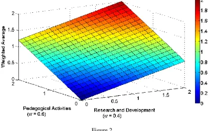
i_ w a ; see [4 or 5].

In our case w w₁, ₂, ,w_m are the weights of the areas of interest and a a₁, ₂, ,a_m are the corresponding (normalized) partial evaluationsPE PE₁, ₂, ,PE_m. This aggregation operator is fairly easy to use and compute. That is why WA is the most commonly used aggregation operator in the existing academic staff evaluation models. However, using this operator, we are unable to appreciate excellent performance and to penalize unsatisfactory performance (see Figure 2).

Figure 2 Weighted Average

Fixed weights for both areas of interest that are the same for all staff members do not allow us to assess people according to their focus (the area they are good in).

Such an evaluation approach motivates people to concentrate on the area with greater assigned weight. (Let us say PA has the weight w=0.6 and RD has the weight w=0.4. Balanced performance represented by the standardized score of 1 for both areas results in the overall evaluation of 1. However if the normalized partial evaluation in PA is 0 and 2 in RD, the overall performance in this case is 0.8. Thus we can see that excellent performance in the activity with lower weight is unable to outweigh balanced performance (with scores 1 and 1) in both areas of activities.)

3.2.2 Ordered Weighted Average (OWA)

Let w w₁, ₂, ,w_m be normalized real weights. Let a a₁, ₂, ,a_m be real numbers.

The mapping OWA:R^mRis called the Ordered Weighted Averaging operator (OWA), if



1, 2, , _m



^m1 _i ( )_i

OWA a a a 



i_ w a _ ^{, where}



 (1), (2), ,( )_m



is a permutation of



^{1, 2, ,m}



such that a_(1)a_(2) a_{( )m} ; see [6].

Again, a a₁, ₂, ,a_m correspond to the normalized partial evaluations

1, 2, , _m

PE PE PE for all the areas of interest. According to the OWA definition, for any i



1, 2,...,m



w_i is the weight assigned to the i-th largest normalized partial evaluation. For our model it holds that w₁w₂ w_m, because we want to reflect (promote) the specialization of academic staff members. As can be easily seen (Figure 3), this approach penalizes balanced performance.

Figure 3 Ordered Weighted Average

Using this aggregation operator we motivate people to specialize but they are free to choose the area (in contrast with the WA, where only specialization in the area with greater weight, assigned by the evaluator, results in better overall evaluation).

If all the staff members wished (and had the skills) to excel in RD, they could all get a good overall evaluation even if there was nobody teaching students and the university failed in one of the key areas.

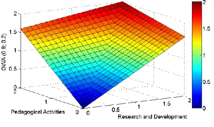
3.2.3 Weighted Ordered Weighted Average (WOWA)

We can combine both previously mentioned aggregation operators into one – the Weighted Ordered Weighted Average (see Figure 4).

Let us consider two sets of normalized real weights w w₁, ₂, ,w_m and

1, 2, , _m

p p p . Let a a₁, ₂, ,a_m be real numbers. The mapping WOWA:R^mRis called the Weighted Ordered Weighted Averaging operator (WOWA), if



1, 2, , _m



^m1 _i ( )_i

WOWA a a a 



i_  a_ ^{, where}



 (1), (2), ,( )_m



is a permutation of



^{1, 2, ,m}



such that a_(1)a_(2) a_{( )m} and _i are defined as

   

* *

( ) ( )

i w j i_ p_ j w j i_ p_ j

 







^{with w*} being a nondecreasing function that interpolates the points

 

^{i m/ ,}

^

^{j iwj}

 

^{,i1, 2, ,m}, together with the point (0,0); see [26].

Using this approach we have two sets of weights available – OWA weights to reflect staff specialisation (again we use w₁w₂ w_m to appreciate staff specialization) and fixed WA weights p p₁, ₂, ,p_m assigned to the areas of interest according to their importance for the success of the university or faculty.

Such aggregation of partial evaluations, however, proves to be too complicated to be understood by the people using the model (executives, heads of departments etc.) and by the academic staff members as well.

Figure 4

Weighted Ordered Weighted Average

Models using WOWA appear “unpredictable” to practitioners as they transform two sets of weights into one, the values of which sometimes surprise the user of the model – we may say that it is not considered “intuitive enough” by the evaluators. The penalization of balanced performance is not removed as well.

3.3 Aggregation of Partial Evaluations by Means of a Fuzzy- Rule-Base System (FRBS)

In order to avoid the penalization of balanced performance, as well as to be able to appreciate excellence on one hand and penalize unsatisfactory performance on the other, a model based on fuzzy linguistic modelling was developed. Another asset of the approach that will be mentioned later in this paper is its comprehensibility, as all the relations between inputs and outputs are described linguistically.

Let us assume that we have available the partial evaluations of PA and RD in terms of multiples of standard scores (for the particular area of interest and work position). Using the tools of linguistic fuzzy modelling, we can now construct a user/evaluator based model – first in a purely linguistic form. Then we assign proper mathematical objects and methods whenever needed using the following algorithm:

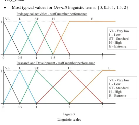
1) We define the set of linguistic terms for the following linguistic variables

 PA (input1): T(PA) = {Very_Low, Low, Standard, High, Extreme},

 RD (input2): T(RD) = {Very_Low, Low, Standard, High, Extreme},

 Overall (output): T(Overall) = {Unsatisfactory, Substandard, Standard, Very_Good, Excellent}.

T(PA), T(RD) and T(Overall) are naturally ordered according to the meanings of the linguistic terms.

2) We define the expected (linguistic) output for each combination of input values (linguistic), thus forming a linguistic rule base containing k rules (25 in our case), such as:

…

If PA is Standard and RD is Standard then Overall is Standard.

If PA is Standard and RD is High then Overall is Very_Good.

If PA is High and RD is Standard then Overall is Very_Good.

If PA is High and RD is High then Overall is Excellent.

…

3) Now we need to specify both input variables regarding the mathematical level of description of their values. As both inputs are mathematically expressed in terms of standard score multiples, the domains for PA and RD are [0,BB] and [0,CC] respectively, where BB and CC are sufficiently high real numbers not to be exceeded by any actual PA and RD partial evaluation respectively.

We define the “most typical” real value of the partial evaluation (in terms of standard score multiples) for each linguistic term of all the inputs defined in step 1):

 most typical values for PA linguistic terms: {0, 0.5, 1, 1.5, 2};

 most typical values for RD linguistic terms: {0, 0.5, 1, 2, 3}.

For the output linguistic variable Overall we define the universe to be [0,2].

We need to define the most typical values of its linguistic terms as well.

These values serve here as category labels. We may see the evaluation process as a classification problem. The information that a staff member is Unsatisfactory in the degree of 0, Substandard in the degree of 0, Standard in the degree of 0.4, Very_Good in the degree of 0.6 and Excellent in the degree of 0 is sufficient. We need to perform a fuzzy classification. To achieve this we assign the key output linguistic terms the values of an ordinal scale: 0 for Unsatisfactory, 1 for Standard, and 2 for Excellent. Meanings of the remaining two linguistic terms are 0.5 for Substandard and 1.5 for Very_Good.

 Most typical values for Overall linguistic terms: {0, 0.5, 1, 1.5, 2}

Figure 5 Linguistic scales

Figure 6

Fuzzy scale describing the overall performance in PA and RD of a current staff member 4) For the input variables PA and RD and for the output variable Overall we

construct (on the respective universes) fuzzy scales using the already defined linguistic terms. The “most typical” values lie in the kernels of these fuzzy numbers (Figures 5 and 6). This way we get

 ⁽PA T PA^{, ( )}



^Very Low Low Standard High Extreme^{_ , , , ,}



^{,[0, BB],}MPA⁾

 ⁽RD T RD^{, ( )}



^Very Low Low Standard High Extreme^{_ , , , ,}



^,[0,CC],MRD⁾

 (Overall T Overall, ( ){Unsatisfactory Substandard Standard Very Good, , , _ , },[0, 2], _Overall)

Excellent M .

The definition of M_PA(Extreme) and M_RD(Extreme) corresponds with the normalization process described previously (see Figure 1).

5) For any pair of real inputs pa[0,BB] and rd[0,CC] we can now compute the output (real) value

1

1 1

( ) ( )

( , ) ( ) ( )

( ) ( )







 

   



 



k

j j j k

j

j j j

k

j

j j

j

A pa B rd ev

eval pa rd A pa B rd ev

A pa B rd

, (4)

where

 Aj is the fuzzy number representing the meaning of the linguistic term describing PA in rule j, j=1, ..., k;

 B_j is the fuzzy number representing the meaning of the linguistic term describing RD in rule j, j=1, ..., k;

 ev_j is the real number representing the most typical value of the linguistic term describing the Overall in rule j , j=1, ..., k; ev_j lies in the kernel of the respective triangular fuzzy number.

As we are using linguistic scales and have only two crisp inputs, no more than 4 rules can be called for at the same time. It is easy to prove that



^kj_1A pa B rd^j( ) ^j( )1. Let A pa₁( ) a 0 and B rd₁( ) b 0,

 

, 0,1

a b , which means that the truth value of this rule is a b . We can find no more than three other rules with non zero truth values, namely:



1 a b



,



¹



a b and



^{1  a}

 

^{1 b}



. The sum of these four truth values is equal to 1.

Formula (4) interpolates the overall evaluation function eval(pa, rd) defined by a finite amount of known values (25 in this case) as shown in Figure 7.

The result is a piece-wise bilinear function. Moreover for all x₁x₂,

1, 2[0, BB]

x x , and y₁y₂, y y₁, ₂[0,CC], it holds that

1 1 2 2

( , ) ( , )

eval x y eval x y . As we have assured that eval is nondecreasing in both arguments for the 25 typical combinations of values (defined in steps 2 and 3), the interpolated function is nondecreasing in both arguments as well.

To linguistically interpret the crisp output eval of step 5, we use the linguistic fuzzy scale Overall. The output can now be interpreted in terms of membership degrees to the fuzzy numbers that represent the meanings of linguistic terms from T(Overall). For example, the overall evaluation 1.2 will be interpreted as 0.6 “Standard” and 0.4 “Very_Good”. This way the fuzzy classification is complete. The result of the algorithm is a description of a current staff member’s performance that uses the predefined five linguistic terms (labels of the categories) and specifies the membership degree of the staff member to each category. Such description is easy to understand and still provides a valuable piece of information.

The linguistic rule base constructed in step 2 describes the aggregation of PA and RD partial evaluations much more transparently than all the previously mentioned models (particularly for laymen). By the use of linguistic fuzzy modelling we have constructed an evaluation tool that is easy to understand, easy to use and even easy to modify for various purposes. Due to the chosen approximate reasoning mechanism, it is computationally undemanding as well. Figure 7 shows the shape of the aggregation function described by the fuzzy rule base. It meets all the requirements concerning excellence appreciation and unsatisfactory performance penalization mentioned in the introduction. The outputs are available as real numbers as well as their linguistic descriptions.

Figure 7

The shape of the linguistically defined aggregation function for PA and RD partial evaluations

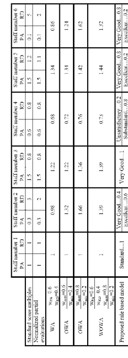
3.4 Numerical Example

Let us consider six academic staff members (SM1,…,SM6). For each of them we have the partial evaluations in terms of multiples of the appropriate standard scores (see Tab. 1). We calculate the normalized partial evaluations as described earlier in the paper (setting excellence at three times the standard score for RD and twice the standard score for PA). All these normalized partial evaluations lie in [0,2], where 1 corresponds to a standard performance and 2 to an excellent performance. To aggregate these partial evaluations, WA, OWA, WOWA, and the fuzzy-rule-base model introduced in this paper were applied.

Staff member 1, who is standard in both areas, is always evaluated as standard regardless of the aggregation method used. Using the WA, SM₂ and SM₆ are evaluated worse than the “standard” SM₁, even though they show excellent performance in RD. By comparing the WA evaluation of SM₁, SM₂ and SM₆, it is obvious that specialization in RD is discouraged, as excellence in RD is unable to outweigh the low performance in PA. Due to the fixed weights, the use of WA can result in classifying people excellent in one of the areas of interest as standard or worse.

This is not the case with the OWA operator, which is able to reflect and appreciate staff members’ specialization, as Tab. 1 clearly illustrates. However, there is no way for the executives to influence the area of specialisation of their staff (by the use of the evaluation model). The WOWA operator solves even this problem but the results of combining two sets of weights defined by the evaluator are not well accepted by laymen. If the partial evaluation in the area with the larger fixed weight is larger than evaluation in the other area (SM₃, SM₅), the resulting aggregated evaluation is larger than those obtained by the use of WA and OWA.

The use of the fuzzy-rule-base evaluation model described in this paper results in a linguistic description of each staff member’s performance. The numerical value of the function eval that results from step 5 in Section 3.3 is also available to the evaluator (its values are 1 for SM_1, 1.8 for SM_2, 1.5 for SM_3, 0.4 for SM_4, 1.6 for SM_5, 1.6 for SM₆). Results provided by the fuzzy-rule-base model (the fuzzy classification of a staff member according to his/her performance in PA and RD) are easy to understand and need no further explanation. The evaluation process is described linguistically, and therefore even staff members themselves can see how the evaluation works.

Conclusions

We have described several mathematical tools that can be used in academic staff performance evaluation for the aggregation of partial evaluations. Having identified the weak spots of the previously discussed aggregation operators, we have suggested a new model that is based on fuzzy-rule-base systems. The main advantage of the proposed model is that it is easy to understand, easy to use and easy to modify to meet the specific requirements of the evaluator. Outputs (evaluations) are available on different levels of aggregation, thus giving an overall picture of a staff member’s performance in a graphical form with linguistic labels, as well as detailed information concerning the performance in all the areas relevant for evaluation. This makes the proposed model, which is currently being implemented at Palacky University, a multipurpose performance assessment tool.

The developed performance evaluation system is beneficial to academic staff members as well – it serves as a record of their activities for their own needs. It provides feedback on their performance (and how the employer sees this performance). Aggregated information available in an easy to understand form is an important management tool for the executives, namely the heads of departments. The long-term use of the model offers the opportunity to observe the dynamics of staff member performance over time, which can be seen as another valuable asset of our model.

Acknowledgement

The research was supported by the grant PrF_2010_08 of the Internal Grant Agency of Palacky University in Olomouc.

References

[1] Chvátalová, A., Kohoutek, J., Šebková, H. (eds.): Quality Assurance in Czech Higher Education (in Czech). Aleš Čeněk, Plzeň 2008, ISBN 978- 80-7380-154-0

[2] European Association for Quality Assurance in Higher Education [online]

<http://www.enqa.eu/>

Table 1 Overview of the results for WA, OWA, WOWA, and FRBS aggregation of partial evaluations

[3] Matheson, W., Van Dyk, C., Millar, K. I.: Performance Evaluation in the Human Services. The Haworth Press, New York-London, 1995. ISBN 1- 56024-379-1

[4] Dubois, D., Prade, H. (Eds.): Fundamentals of Fuzzy Sets. The Handbook of Fuzzy Sets Series. Kluwer Academic Publishers, Boston-London- Dordrecht. 2000. ISBN 0-7923-7732-X

[5] Torra, V., Narukawa, Y.: Modeling Decisions. Springer, Heidelberg, 2007.

ISBN 978-3-540-68789-4

[6] Yager, R. R.: On Ordered Weighted Averaging Aggregation Operators in Multicriteria Decision Making. IEEE Trans. On Systems, Man and Cyberneics 3 (1) 1988, pp. 183-190

[7] Talašová, J.: Fuzzy Methods of Multiple Criteria Evaluation and Decision Making (in Czech) Palacky University, Olomouc, 2003, ISBN 80-244- 0614-4

[8] 2009-10 Guidelines for Evaluation of Academic Staff [online] Wayne State University [cited 30. 5. 2010]

<http://www.aaupaft.org/pdf/AcStaffguidelines_2009-10.pdf>

[9] Academic Performance Evaluation [online] c2010, last revision May 15, 2010, McGill University [cited 30. 5. 2010]

<http://www.mcgill.ca/medicine-academic/performance/>

[10] Performance Management [online] c2009, University of Technology Sydney [cited 30. 5. 2010] <http://www.hru.uts.edu.au/performance /reviewing/rating.html>

[11] Performance Management [online] Flinders University [cited 30. 5. 2010]

<http://www.flinders.edu.au/ppmanual/review.html>

[12] Determination of Criteria for Pedagogical and Other Activities Evaluation (in Czech) [online] Brno, Masaryk University, Faculty of Law [cited 30. 5.

2010]. <http://www.law.muni.cz/dokumenty/7601>

[13] Academic Staff Evaluation Criteria for Personal Extra Pay Distribution (in Czech) [online] Ústí nad Labem, Jana Evangelista Purkyne University, Faculty of Environment [cited 30. 5. 2010]

<http://fzp.ujep.cz/dokumenty/kritosoh.pdf>

[14] Pedagogical and Creative Activities Evaluation (in Czech) [online] Zlín, Tomas Bata University in Zlín, Faculty of Applied Informatics [cited 30. 5.

2010] <http://web.fai.utb.cz/cs/docs/SD_09_09.pdf>

[15] Talašová, J., Pavlačka, O.: Academic Staff Evaluation Model Design for the Faculty of Science, Palacky University in Olomouc (in Czech) Research report. Faculty of Science, Palacky University, Olomouc 2006

[16] Talašová, J., Stoklasa, J., Pavlačka, O., Holeček, P.: New Academic Staff Evaluation Model Design for the Faculty of Science, Palacky University in Olomouc (in Czech) Research report. Faculty of Science, Palacky University, Olomouc 2009

[17] Mamdani, E. H., Assilian, S.: An Experiment in Linguistic Synthesis with a Fuzzy Logic Controller, Int. J. Man-Machine Studies, Vol. 7, 1975, pp. 1- 13

[18] Sugeno, M.: An Introductory Survey on Fuzzy Control. Information Sciences, 36, 1985, pp. 59-83

[19] Zadeh, L. A.: Fuzzy Sets. Inform. Control, 8, 1965, pp. 338-353

[20] Ruspini, E.: A New Approach to Clustering. Inform. Control, 15, 1969, pp.

22-32

[21] Codara, P., D’Antona, O. M., Marra, V.: An Analysis of Ruspini Partitions in Gödel Logic. International Journal of Approximate Reasoning, 50, 2009, pp. 825-836

[22] Zadeh, L. A.: The Concept of Linguistic Variable and its Application to Approximate Reasoning. Information Sciences, Part 1: 8, 1975, pp. 199- 249, Part 2: 8 1975, pp. 301-357, Part 3: 9 1975, pp. 43-80

[23] Takagi, T., Sugeno, M.: Fuzzy Identification of Systems and its Application to Modeling and Control. IEEE Transactions on Systems, Man and Cybernetics, 1 (15), 1985, pp. 116-132

[24] Sugeno, M., Yasukawa, T.: A Fuzzy-Logic-based Approach to Qualitative Modeling. IEEE Transactions on Fuzzy Systems, 1 (1), 1993, pp. 7-31 [25] Methodology for Research and Development Outcomes Evaluation (in

Czech) [online] Research and Development in the Czech Republic [cited 30.5. 2010], http://www.vyzkum.cz/storage/att/CDDC542199F1640B59A 7D1E84 1B7151C/Metodika%202009_schv%c3%a1leno.pdf

[26] Torra, V.: The Weighted OWA Operator. International Journal of Intelligent Systems. 2 (12), 1997, pp. 153-166

[27] Babak Daneshvar Rouyendegh, Serpil Erol: The DEA – FUZZY ANP Department Ranking Model Applied in Iran Amirkabir University, in Acta Polytechnica Hungarica, Vol. 7, No. 4, 2010, pp. 103-114

[28] Lívia Róka-Madarász: Performance Measurement for Maintenance Management of Real Estate, in Acta Polytechnica Hungarica, Vol. 8, No. 1, 2011, pp. 161-172