Construction of a Realistic Signal Model of Transients for a Ball Bearing with Inner Race Fault

(1)

Construction of a Realistic Signal Model of Transients for a Ball Bearing with Inner Race Fault

Lajos Tóth

Department of Electrical and Electronic Engineering University of Miskolc

H-3515 Miskolc-Egyetemváros, Hungary e-mail: elklll@uni-miskolc.hu

Tibor Tóth

Department of Information Engineering University of Miskolc

H-3515 Miskolc-Egyetemváros, Hungary e-mail: toth@ait.iit.uni-miskolc.hu

Abstract: This paper considers the creation of a transient vibration signal model established for signals generated in deep grove ball bearings with pitting (spalling) formulation on their inner race. The fault on the inner race was created artificially. The derivation of the signal model is based on data acquisition, signal filtering and parametric identification. A new filtering method is presented that is suitable to eliminate the effect of amplitude modulation and noise that usually arises in the case of bearing vibration measurements. We show that a three-parameter signal model is adequate to describe unmodulated transient pulses. Our signal model can be used in developing new bearing vibration analysis and condition monitoring methods.

Keywords: Condition monitoring; bearing vibration analysis; model identification

1 Introduction

Nowadays, bearings are commonly used components in machinery. This component plays a prominent role in the operation of devices. Failure can therefore not only cause enormous damage, but sometimes put human lives at risk.

The failure of rolling element bearings during operation is indicated by the

(2)

L. Tóth et al. Construction of a Realistic Signal Model of Transients for Ball Bearing with Inner Race Fault

unusual behaviour of the bearings. Improper operation may be indicated by a rising or increased vibration level in a bearing. The initial state of "unusual behaviour" is usually followed by sudden failure of the bearings. In this way bearing failures may have unforeseen consequences, and therefore the periodic inspection, preventive maintenance and replacement of defective parts is important.

In order to avoid unexpected failures, various procedures have been developed.

These include condition monitoring and vibration analysis. All of these methods strongly rely upon the kinematical or dynamic model of the bearing. At the early stage of bearing failure, micro-cracks develop under the rolling surfaces due to the repetitive load on the contacting elements. This usually produces high-frequency (ultrasonic) vibrations that can be sensed by acoustic emission methods. In the next phase of bearing failure, these cracks reach the surface. When two surfaces contact each other in this situation, resonance is excited in the bearing.

The mathematical model of the vibration response of the bearing with a single point defect is investigated in [1, 2, and 3]. The authors in [1 and 2] consider the propagation path of the vibration and the effect of load distribution. This type of mathematical model is an exponentially damped sinusoid function. Later, in [4, 5], the signal model was extended to cases of multipoint defect.

Another approach is to model the bearing as many degrees of freedom (DOF) system. The authors in [6, 7 and 8] use a 2 DOF model, while others in [9] a use 3 DOF model. These models are based on the Hertzian contact theory, considering the centrifugal load effect and the radial clearance.

Our aim was to develop a realistic signal model of vibration response of a bearing with a single-point defect by creating an artificial fault. We set up test equipment to record the vibration response of this type of defect, and we also created a model with an appropriate numbers of unknowns and tried to find numerical values to fit these variables by parametric identification, where the measured and the theoretical vibration response are in good agreement.

2 Establishing a Vibration Signal Model

Vibrations generated by bearings appear at different frequency ranges.

Periodically occurring transient pulses are produced at frequencies determined by bearing geometry and speed. The frequencies of transient pulses depend on the characteristic frequencies of the bearing. There are also low frequency vibrations originating from unbalancing. The subject of our examination is the model of these transient pulses.

(3)

2.1 Bearing Selection and Data Acquisition

The primary consideration at bearing selection was its applicability for testing. We had to choose a bearing that can be disassembled and assembled without destruction. Taking into account the available resources and above considerations, a 6204-type, plastic cage, single row, deep groove radial ball bearing was chosen (see Fig. 1).

Figure 1

An assembled and disassembled deep-groove ball-bearing, type 6204

In order to obtain a signal model, we had to form a point-wise fault on the surface of the inner ring of the bearing. Since bearing material is very hard (HRC 58-65), we experimented with applying sulphuric acid and nitric acid on the surface, but in neither case was the fault point wise. Finally, we were able to form a single- point fault (Fig. 2) with an electric arc engraver and with a laser engraver-cutter.

The shape of the failure created by electric arc differs from the ideal circle, while by using a laser beam a hole can be created that is very close to the ideal circular shape. The artificially created fault on the inner race of a deep grove ball bearing is shown in Fig. 3.

Figure 2

The “crater” formed on the inner race of the bearing by electric arc (left) and by laser beam (right)

(4)

Figure 3

An artificially created fault on the inner race of a deep grove ball bearing

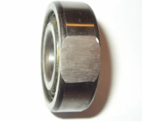
Figure 4 The machined outer ring

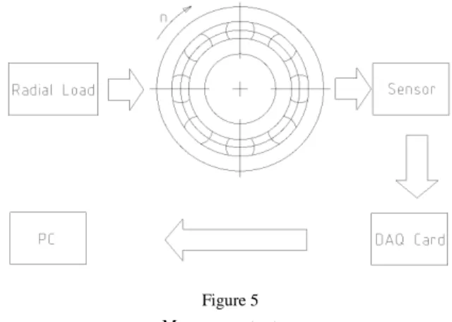
For the test rig we used a turning machine of E1N type. The bored and reassembled bearing was mounted on a shaft fixed in the chuck. We used a rod fixed in the tool post as a support. The rotating nature of the tool post made it possible to apply radial load on the outer ring of bearing, where the force was set to be perpendicular to the rotating shaft. Our primary goal was to minimize the force/vibration transmission path, since noise can come from a number of different sources. They can be mechanical or electrical noises. Electrical noise can be eliminated by properly set up measurement devices, while mechanical noise usually comes from the test rig. A portion of the outer ring of the bearing was machined by grinding (Fig. 4). An accelerometer of KISTLER 8702B50 type was attached to the flat area with beeswax.

(5)

Figure 5 Measurement set up

For data acquisition we used the following devices:

• HAMEG, HM507 analogue-digital oscilloscope, 100 Ms/s real-time sampling rate,

• KISTLER accelerometer 8702B50,

• KISTLER 5108 charge amplifier,

• PCI 6063E PCMCIA DAQ card, 500 ks/s sampling rate.

The DAQ card was controlled by software developed under the NI LabWindows/CVI programming environment. Validation of our software was performed using a HITACHI VG-4429 function generator and digital oscilloscope.

Sampling was performed at a constant inner ring speed of 1812 min^-1. This value satisfies the specifications of American ANSI [10] and German DIN [11]

standards (1800 min^-1 ± 2%) concerning bearing vibration measurements. The outer ring was stationary, as it delivered radial load. The sampling frequency and gain were set to be 30 kHz and unity, respectively.

When a ball rolls over the fatigue point, it excites resonance in the bearing at one of the natural frequencies. The amplitudes of excited impulses are proportional to the load and influenced by the load distribution factor. The closer a fault is located to the load zone, the higher the amplitude of excited impulse is. The repetition frequency of impulses is 30.2 Hz and the time between successive impulses is T=33 ms. The resonance excited by an impact embedded in noise and the corresponding spectrum are plotted in Fig. 6. Since our test rig contains a gearbox to transmit power from the motor to the lathe spindle, the gear mesh frequencies should appear in the spectrum. These frequencies occupy the higher frequency ranges of the spectrum. Using a faultless test bearing of the same type as a reference gauge we were able to distinguish between gear mesh and bearing frequencies.

(6)

Figure 6

Time plot and corresponding amplitude spectra of the bearing with inner race fault

Bearing defect frequencies could also be calculated from the geometry, which is shown in Table 1.

Table 1

Bearing defect frequencies of 6204 bearing for n =1812 min^-1, stationary outer ring BPFI 149.339 Hz

BPFO 92.261 Hz

BSF 60.349 Hz

FTF_i 11.533 Hz

We used a 6th-order Butterworth 300-1800 Hz band-pass filter to remove the unwanted “noise”.

The signal at the output stage of filter still contains a considerable amount of noise. To establish the signal model of this kind of bearing failure we need a

“noiseless” time signal. To resolve this problem we created a new filtering method that used a priori information about the signal.

(7)

Figure 7

Time plot and corresponding amplitude spectra of the faulty bearing after filtering

2.2 Examination of Bearing Vibration Signals

Bearing vibration signals, especially those which result from pitting formulation, are a series of amplitude modulated transient pulses. The source of amplitude modulation is the load distribution, which is unequal along the inner or outer ring of bearing (Fig. 8). The load distribution (Equation (2)) is expressed in terms of the load distribution factor ε. The external radial force generates a number of reactive forces whose amplitude varies with the contact function in Eq. (1). That is, the closer the fault (pitting) is located to the load zone, the higher the amplitude of the transient vibration is.

In case of ε < 1 the load zone can be characterised by the contact function Ψe [12].

(

^ε

)

=

Ψe arccos1−2 ₍₁₎

The load on a rolling element at arbitrary Ψeangle is given as:

( ) (

¹ ^cos

)

^,

2 1 1

max

n

Ψ Ψ

=Q ε

Q 



−

⋅

−

⋅

(2) where Q_maxis the maximum load on a rolling element [12], n=3/2 for bearings with point contact (ball bearings), and n=10/9for bearings with line contact (roller bearings).

(8)

Figure 8

Interpretation of load distribution factor ε [12]

On the basis of static balance, the vertical components of rolling element load should be equal to the external radial load:

( )

^.

cos

0

Q Ψ

= F

Ψ=±Ψe

Ψ=

r

∑

Ψ

(3) Therefore,

( )

( ¹ ^cos ) ^cos ( ) ^.

2 ε 1 1

0

Ψ Ψ

Q

= F

±Ψe Ψ=

Ψ=

n max

r

∑ _ ^ − ⋅ − _ ^

(4) Applying Newton’s second law on (4), i.e. that the acceleration is parallel and directly proportional to the net force, it is clear that the instantaneous amplitudes of vibration acceleration are determined by the radial load corresponding to contact function. That means amplitude modulation.

2.3 Filtering of Amplitude Modulated Transient Pulses

Transient signals are finite energy signals by definition (5)

( ) ^,

∫

2

∞

−

∞ dt<

t x

E=

⁽⁵⁾

where E denotes the energy of signal x(t).

(9)

For characterising those in the time domain, parameters such as rise-time, overshoot, settling-time or fall-time can be used. The shorter its time extent, the wider space it occupies from the frequency plane:

( ) ^δ ^(t) ⁼ ¹ ^,

₍₆₎

where ( ) denotes the Fourier transform operator and δ(t) is the Dirac delta function.

Real world electrical signals are usually embedded in noise. In the case of vibration measurements we convert the mechanical displacement into voltage.

Noise might come from the equipment where the investigated part is located. This usually happens, even if it operates under normal condition. Noise can also be measurement noise that arises during the converting process of mechanical quantities into electrical values. Or it might originate from EMC disturbances. But it can also be quantization error arising during A/D conversion.

Depending on the source of the noise, its spectrum may be located within a specific frequency area or it might occupy the whole frequency range. The filtering of transient signals embedded in noise by conventional methods is difficult, since it is hard to establish the cut-off frequencies of the filters accurately.

In certain engineering processes, periodically repeated transient impulses arise whose amplitude varies with time depending on some physical parameters. This means that the transient impulses amplitude is modulated. The amplitude modulation alters the original pulse spectrum. The location of sidebands depends on the modulation index and the shape of modulating signal. In addition, this spectrum is usually buried in one of the previously mentioned noises, depending on the signal to noise ratio (SNR).

Assuming that each transient impulse is just as likely to appear in the sampled data, and its time course – aside from the differences caused by amplitude modulation – is the same, we obtain the most accurate frequency domain representation if we take as many samples of the pulse as possible. If the transient pulses are generated by a deterministic process, the repetition rate is constant or well defined.

The Fourier transform of absolutely integrable finite-energy signals with only a finite number of local extremes is a continuous function. Amplitude spectra of periodic functions are line spectra, where the distance between individual spectral lines is equal to the frequency calculated from the periodicity. As a result, the Fourier transform of periodically recurring transient signals must be line spectra.

When a periodic signal is amplitude modulated, side bands appear in its spectra.

The spectral line corresponds to the carrier signal and the sidebands to the modulating frequency, respectively.

(10)

One form of amplitude modulation (AM-DSB, or A3E) in time-domain can be written as:

( ) ^t ⁼ [ ^A ⁺ ^m ( ) ^t ] ^c ( ) ^t

x ⋅

^, ₍₇₎

where x(t) is the amplitude modulated signal, m(t) is the information (modulating signal, base band signal), c(t) is the carrier and A is a constant.

The general form of the carrier signal

( ) t C ^sin (

c

t

c

) ^,

c = ⋅ ω + φ

₍₈₎

where C, φc and ω_care the amplitude, phase and angular frequency of the carrier.

The time function of the modulating signal

( ) ^t ⁼ ^M ^⋅ ^cos ( ^ω ^t ⁺ ^φ ) ^,

m

_m

(9) where M is the amplitude maxima of the modulating signal, and φ^and^ωm are the phase and angular frequency of the modulating signal.

The carrier and the modulating signal frequency can be calculated based on Equations (10) and (11).

π ω 2

c

f

c

=

(10)

π ω 2

m

f

m

=

(11) The carrier frequency is always greater than the frequency of the modulating signal:

m

c

f

f >>

_. ₍₁₂₎

If A=0 then we have double-sideband suppressed-carrier transmission (DSBSC).

The condition of double-sideband amplitude modulation: A ≥ ^M.

The modulation depth can be calculated using

A m= M

(13) Assuming an additive, uniformly distributed "white noise" e(t) with zero mean, the amplitude modulated signals embedded in noise can be written in the form:

( ) ( ) ( ) +

(11)

White noise is a signal where the consecutive samples do not correlate:

( ) ( )

{ }

 



≠

= =

2 1

2 1 , 2 2

*

1

0 ,

2

,

1

t t

t t t

e t e

E σ δ

^t ^t

, (15)

where E{e(t)} is the expected value of random variable e(t) (mean value, average value) and the asterisk stands for the complex conjugation

σ²^=E{|^e(t)|²} variance of random variable e(t) (power).

The autocorrelation function of a white noise is a pulse at t₁ = t₂.

Since the Fourier transform of the autocorrelation function is the power spectral density (PSD), PSD of the white noise is constant throughout the entire frequency range. This means that all frequencies are present in the white noise:

( )

{ e t } = σ

e²

^.

₍₁₆₎

The Fourier transform of a noisy, amplitude modulated signal is

( )

{ ^y ^t } ⁼ ^A { ^c ( ) ^t } ⁺ { ^m ( ) ( ) ^t ^c ^t } { ^e ( ) ^t } ^,

⋅ ⋅ +

₍₁₇₎

where the first part of the right side of the equation is the Fourier transform of the carrier, the second part is the Fourier transform of the modulated carrier, and the third part is the PSD of white noise. The Fourier transform of the second term in Equation (17) can be calculated as follows:

( ) ( )

{ } ^ˆ ( ) ( ) ^ˆ ^,

2 1 m ω c ω π

= t c t

m ⋅ ⋅

(18)

where the hat denotes Fourier transformation.

The harmonics in this term are symmetrical to the higher-frequency carrier. Those harmonics which correspond to the carrier are missing from the spectra.

Using Equation (18) we see that

( ) ( )

{ } [ ( ⁴ ) ( ² ) ( ² ) ( ⁴ ) ] ^.

2 1 − + + + − + +

⋅ c t = π δ w δ w δ w δ ω

t m

(19) The first part of the right side of Equation (17) represents transient pulses.

( ) ⁼ { ^c ( ) ^t }

C ^ˆ ω

₍₂₀₎

This term gives line spectra, since we have periodic function. The distance between successive spectral lines is the aforementioned repetition frequency.

If the amplitude or the frequency of modulating signal changes with time, then the position of spectral lines representing carrier frequencies in Equation (17) does not

(12)

change, but the amplitude of side bands (second term) and their distance from the carrier also alter. The location of the sidebands is determined by the modulating signal.

( ) { ^m ( ) ( ) ^t ^c ^t }

M ^ˆ ω = ⋅

₍₂₁₎

Using Equation (12, 18 and 19) Equation (17) can be rewritten as (22)

( ) ^ˆ ( ) ( ) ^ˆ ^.

ˆ

²

M

e

+ C A

=

Y ω ⋅ ω ω + σ

₍₂₂₎

The second term containing modulation information from Equation (22) by spectral sampling can be removed, since it has no spectral component corresponding to the carrier frequency:

( ) ∑ (

⁻ ^⋅^∆

) ( )

^⋅ ^∈^Ζ

=

n Y f n

= Y

N

n

s ˆ ,

ˆ

0

ω ω

δ

ω

⁽²³⁾

where Yˆs

( )

ω denotes the sampled spectra, Z denotes the set of integer numbers, and ∆f is the periodicity we get from Cepstral analysis:

( )

^,

log ˆ 2

] 1

[

ω

τ π

^π ^ω^τ

π

ω e d

e Y ^j ^j

∫

−

=

(24)

( )

^τ

[ ] ( )

^τ

τ where c c

f = , =max

∆ _. ₍₂₅₎

To determine the frequency domain form of transient pulses we can use:

( )

¹ ^ˆ ²

ˆ Ys e

=A

Cω −σ

(26) The value A is a constant determined by the amplitude of the modulating signal.

When it is unknown, then let A = 1. The filtered transient pulses can be obtained by using inverse Fourier transformation

( )

^t

{ }

^C

( )

^ω

c =⁻¹ ˆ

. (27)

The proposed method consists of:

− sampling, considering Shannon’s theorem.

− performing Cepstral analysis to determine periodicities in the spectra.

− estimating the noise level using signal spectra.

− sampling the amplitude spectra, according to the results of Cepstral analysis.

− decreasing the amplitude values by the estimated noise level

(13)

2.3.1 Application of the Method for Filtering Bearing Vibration Signals In our case transient pulses correspond to the carrier wave, while the effect of amplitude modulation caused by load distribution factor corresponds to the modulating wave (Fig. 9). Applying the filtering method on sampled data of vibration of laser drilled bearing, we were able to eliminate the effect of amplitude modulation. The time-domain behaviour of each transient in the filtered signal is the same, which makes it possible to establish a signal model of transient vibration for this type of bearing failure.

Figure 9

Filtered vibration acceleration signals of the laser drilled bearing

2.4 Model Identification

Model identification can be performed in various ways. Our main idea was signal enveloping followed by curve fitting. Since the transient signal of this type of defect does not contain a frequency modulated component (see Fig. 12), all we have to be concerned with is the amplitude modulating element.

In [3, 12] the signal model of transient pulse generated by a point-wise fault on the inner race of a deep groove ball bearing is defined as an exponentially damped sine function

( ) ^t ^A ^e ^sin ( ^t ) ^,

x = ⋅

⁻^C^⋅^t

⋅ ω

_n

⋅

₍₂₈₎

(14)

where

ω

_n

= ² π f

_n^{, f}n is the n^th natural frequency of bearing system, C is a damping factor, and A is the initial amplitude.

We created our signal model using a priori knowledge of the process. The idea is that the transient pulse can be decomposed into two parts: one that is responsible for the amplitude rise and decay of the transient in time, and one that corresponds to one of the natural frequencies of the bearing. Our signal model consists of product of these terms:

( ) ( ) ( )

^t ^m^t ⁿ^t ^,

x = ⋅ ₍₂₉₎

where m(t) is the amplitude modulating part and n(t) is the frequency modulating part.

To determine the envelope function m(t) we calculated the magnitude of the Hilbert transform of the sampled and filtered transient:

( )

^t

{

^x

( )

^t

}

^,

m = ⁽³⁰⁾

where { } denotes the Hilbert transform operator.

The time plot of the sampled and filtered transient and its envelope is shown in Fig. 10.

Equation (28) assumes a sudden rise in the transient pulse. This may be a valid way of describing a process in which the excitation of material with shock pulse and test of the response is within the same material. The transient pulse emitted by a ball rolling into the fault triggers a series of plastic deformation. Our signal model takes into account the transient formulation and decay process. We assumed that, if coefficients used in our signal model fit well with the envelope of the transient, the signal model can be considered appropriate.

We searched the equation of demodulated transient in the form of the following:

( ) ^t ⁼ ^A ^⋅ ^t ^⋅ ^e

⁻ ^⋅

^, ^t ^∈ ^[ ⁰ ^, ^∞ ^), ^A ^, ^C ^, ⁿ ^∈ ^ℜ ^,

m

ⁿ ^C^t ₍₃₁₎

where A, C, n are process parameters and ℜ denotes the set of real numbers.

(15)

We used the Nelder-Mead non-linear simplex method to find the best-fit parameters A, n and C that minimize the Mean Squared Error (MSE). The calculated best-fit parameters are shown in Table 3.

Table 3

Best-fit parameters for the demodulated transient in Equation (31) A 5.5749e-6

n 1.8334

C 0.008

MSE 1.8729e-5

The result of the curve fitting process can be seen in Figure 11.

Figure 11

The envelope plot of sampled and approximated data

The curve obtained by approximation displays an adequate fit with the envelope of the sampled and filtered data. Because we were able to find parameters with which our equation well approximates the envelope of the sampled and filtered transient, our signal model can be considered appropriate. We performed the same fitting process with four variables. The result showed that value of the fourth variable was very close to one. Thus we considered the three-parameter model appropriate.

Figure 12

Instantaneous-frequency plot of the transient

(16)

To examine the behaviour of the transient in the frequency domain, we calculated the instantaneous-frequency values.

It can be seen in Figure 12 that the instantaneous frequency hardly changes with time. This means that the transient is not modulated in frequency. This gives the second part of (29) in the following form:

( ) ^t ^sin ( ^t ) ^,

n = ω

_n

⋅

₍₃₂₎

where

ω

_n

= ² π f

_n^{, f}n and is one of the natural frequencies of the bearing.

2.5 Model Verification

We used the vibration samples of a faulty bearing of type 6209 to validate our model. After filtering and demodulating the transient we performed the same fitting process as before. We were able to find coefficients which gave reasonable error (Table 4).

Table 4 The best-fit parameters A 1.0065e-10

N 4.583

C 0.0114 MSE 0.2765

The time plot of the sampled transient pulse of vibration signal of the laser-drilled bearing and its approximated envelope function are shown in Fig. 13.

Figure 13

Time plot of sampled signal and simulated transient signal model

(17)

3 The Proposed Signal Model

Our studies have shown that our signal model (Eq. (33)) can be used to describe the signal caused by a point-like defect on the inner race of a deep groove ball bearing.

( ) ^t ⁼ ^A ^⋅ ^t ^⋅ ^e

⁻ ^⋅

^⋅ ( ^⋅ ^t ) ^t ^∈ ^∞ ^A ^C ⁿ ^∈ ^ℜ

x

ⁿ ^C^t

sin ω

_n

, [ 0 , ), , ,

⁽³³⁾

where

ω

_n

= ² π f

_n^{, and f}n is one of the natural frequencies of the bearing.

Table 5

Model parameters of Equation (35) A 5.5749e-6

n 1.8334

C 0.008

For simulation purpose the values shown in Table 5 can be used. But care should be taken as these values change with load.

Conclusions

In this paper we developed a new signal model for a point-wise fault on the inner race of a deep grove ball bearing. A new filtering method was presented which is suitable for eliminating the effect of amplitude modulation and noise that usually arise in the case of bearing vibration measurements. We showed that a three- parameter model is adequate to describe the transient pulses. This model, however, does not take into account the magnitude of the load. By doing so it would be possible to give quantitative values of the model parameters. Our signal model can be used in developing new analysis methods.

Acknowledgement

This research was carried out as part of the TAMOP-4.2.1.B-10/2/KONV-2010- 0001 project with support by the European Union, co-financed by the European Social Fund.

References

[1] McFadden PD, Smith JD., Model for the Vibration Produced by a Single Point Defect in a Rolling Element Bearing, Journal of Sound and Vibration 96 (1984), pp. 69-82

[2] N. Tandon, A. Choudhury, An Analytical Model for the Prediction of the Vibration Response of Rolling Element Bearings due to a Localized Defect, Journal of Sound and Vibration, Vol. 205 (1997), pp. 275-292 [3] S. Ericsson, N. Grip, E. Johansson, L.-E. Persson, R. Sjöberg, J.-

O.Strömberg: Towards Automatic Detection of Local Bearing Defects in

(18)

Rotating Machines, Mechanical Systems and Signal Processing 19 (2005) pp. 509-535

[4] P. D. McFadden, J. D. Smith, The Vibration Produced by Multiple Point Defects in a Rolling Element Bearing, Journal of Sound and Vibration, Vol.

98 (1985) pp. 263-273

[5] A. Choudhury, N. Tandon, A Theoretical Model to Predict Vibration Response of Rolling Bearings to Distributed Defects under Radial Load, ASME Transactions Vol. 120 (1998) pp. 214-220

[6] C. S. Sunnersjo. Varying Compliance Vibrations of Rolling Element Bearings. Journal of Sound and Vibration, Vol. 3 (1978) pp. 363-373 [7] A. Rafsanjani, S. Abbasion, A. Farshidianfar, and H. Moeenfard. Nonlinear

Dynamic Modeling of Surface Defects in Rolling Element Bearing Systems. Journal of Sound and Vibration, Vol. 319 (2009) pp. 1150-1174 [8] M. Tadina, M. Boltezar, Improved Model of a Ball Bearing for the

Simulation of Vibration Signals due to Faults during Run-up, Journal of Sound and Vibration, Vol. 330 (2011) pp. 4287-4301

[9] H. Arslan and N. Akturk. An Investigation of Rolling Element Vibrations Caused by Local Defects. Journal of Tribology, Vol. 130 (2008), pp. 1-12 [10] American National Standard ANSI/AFBMA Std 13-1970, ANSI B3.13-

1970, Rolling Bearing Vibration and Noise (Methods of Measuring) [11] Deutsches Institut für Normung DIN 5426, Laufgeräusche von Wälzlagern,

Prüfverfahren

[12] L. Molnár and L. Varga: Gördülőcsapágyazások tervezése (Roller Bearings Design), Műszaki Könyvkiadó, Budapest, 1977 (in Hungarian)

Construction of a Realistic Signal Model of Transients for a Ball Bearing with Inner Race Fault