Zolta´nSzabo´ LPV SYSTEMS A GEOMETRICAPPROACHFORTHECONTROLOFSWITCHEDAND

(1)

A GEOMETRIC APPROACH FOR THE CONTROL OF

SWITCHED AND LPV SYSTEMS

by

Zolta ´n Szabo ´

Ph.D.

A DISSERTATION SUBMITTED IN PARTIAL FULFILLMENT OF THE REQUIREMENTS FOR THE DEGREE OF

D.Sc.

AT

H

UNGARIAN

A

CADEMY OF

S

CIENCES

Budapest

2010

(2)

Zolta´n Szabo´, PhD

Systems and Control Laboratory

Computer and Automation Research Institute Hungarian Academy of Sciences

H-1111 Budapest, Kende u. 13-17.

Hungary

A geometric approach for the control of switched and LPV systems

1. Switched systems 2. Geometric system theory 3. Bimodal systems 4. Dynamic inversion Typesetting in L^ATEX2: Camera ready by the author

c Zolta´n Szabo´ 2010 ALLRIGHTSRESERVED.

(3)

Acknowledgements

The thesis contains the results of an intensive research activity performed during the last decade.

Throughout his work the author has been supported by many people, especially by the members of the Systems and Control Laboratory (SCL) of Computer and Automation Research Institute of the Hungarian Academy of Sciences (MTA-SZTAKI). Special thanks to MTA-SZTAKI which provided excellent conditions of research which helped to accomplish this work in the defined quality.

The author is deeply indebted to Prof. Jo´zsef Bokor whose stimulating suggestions and encouragement was indispensable during this period. The author would like to express his sincere gratitude to Prof. Tibor Va´mos and Prof. La´szlo´ Keviczky academicians their encouraging remarks and for the many useful comments. Discussions with Prof. Rudolf E. Kalman and Prof. Michael Athans have a great impact on the scientific view of the author. The stimulating personal commu- nications with Prof. Gary Balas, head of the Department of Aerospace and Mechanics, University of Minnesota were always a source of encouragement for the research.

The author expresses his gratitude to all members of SCL. Special thanks to Dr. Pe´ter Ga´spa´r for the fruitful discussions and valuable suggestions that considerably improved the content and presentation quality of this work. The author is also grateful to Prof. Ferenc Szigeti for the fruitful discussions along the interesting mathematical aspects of the research.

It is also to be noted that the research has been supported by various grants and organizations.

Special thanks to the Hungarian Scientific Research Fund (OTKA), the National Research and Development Foundation (NKFP) which supported projects between 2000 and 2008, the NASA Langley grant with Dr. Christine M. Belcastro as technical monitor, the grant of the Air Force Office of Scientific Research, Air Force Material Command, USAF (EOARD) with Dr. Paul Losiewicz as technical monitor, and the support of the National Science Foundation.

(7)

1 Introduction

In general terms, control theory can be described as the study of how to design the process of influencing the behavior of a physical system to achieve a desired goal. Anopen-loop controlis one in which the control input is not affected in any way by the actual (measured) outputs. If the system changes during the operational time then thecontrol performancecan be severely reduced. In aclosed- loop systemthe control input is affected by the measured outputs, i.e., afeedbackis being applied to that system. Very often a reference input is given, which is directly related to the desired value of system outputs, and the purpose of the controller will be to minimize the error between the actual system output and the desired (reference input) value.

While construction of automatic machines dates back at least to the time of ancient greeks,

Heron of Alexandria as far as automatic control is concerned, a historical example

cited in many texts is James Watt’s fly-ball governor from the 18^th century, where the control objective is to ensure that the speed of rotation is approximately constant. As the fly-balls rotate so they determine, via the valve, how much steam is supplied; the faster the rotation – the less steam is supplied. The rate of steam supplied then gov- erns, via the piston and flywheel, the speed of rotation of the fly-balls. Although tight limits of operation, in terms of speed variation, can be obtained with such a device a possible disadvantage of the feedback scheme is shown: oscillations can occur in the system output, i.e., the speed

of rotation, which would not occur if the system were connected in open-loop mode.

MEASURED SPEED GOVERNOR

VALVE

OUTPUT SHAFT

ENGINE

1

Watt’s regulator

In the second half of the 19^th century J. C. Maxwell developed a theoretical framework for such regulators by means of a differential equation analysis relating to performance of the overall system, thereby explaining in mathematical terms reasons for oscillations within the system. It was gradually found that Maxwell’s gover- nor equations were more widely applicable and could be used to describe phenomena in other systems, an example being piloting (steering) of ships.

A common feature with these systems was the employment of information feedback in order to achieve a controlling action, an idea that was widely exploited in the technological achievements of the 20^th century. As usual, armed conflicts has a great impact on the technological innovation and the last century was not in need of such opportunities. In particular, the Second World War provided an ideal breeding

(8)

1 Introduction

ground for further developments in automatic control. In this period was developed theclassical controltheory, represented, among others, by the work of H. W. Bode, A. Kolmogorov, H. Nyquist, L. Pontryagin and N. Wiener that rely heavily on the spectral properties of the signals and reflects frequency-domain concepts.

In the1960s the influence of space flight was felt, with optimization techniques gaining in promi- nence, while digital control also became widespread due to computers.Modern control theoryhas been developed to cope with the increasing complexity of multiple-input-multiple-output (MIMO) control systems. Unlike classical control theory that is based on frequency-domain analysis, modern control theory is based on time-domain analysis and synthesis using state variables.

R. E. Kalman was the leader in the development of a rigorous theory of control systems. His research in fundamental systems concepts, such as the formulation and study of most fundamental state-space notions, controllability and observability, helped put on a solid theoretical basis some of the most important engineering systems structural aspects. While some of these concepts were also encountered in other contexts, such as optimal control theory, it was Kalman who recognized the central role what they play in systems analysis. The paradigms formulated by Kalman and the basic results he established have become an intrinsic part of the foundations of control and systems theory. The author of this thesis has had the opportunity to meet professor Kalman during his regular visits at MTA SZTAKI. The discussions with him on the topics related to controllability have made a great influence on the research.

There are two main features in the analysis of a control system: system modeling, which means expressing the physical system under examination in terms of a model (or models) which can be readily dealt with and understood, and the design stage, in which a suitable control strategy is both selected and implemented in order to achieve a desired system performance. Forming a mathematical model which represents the characteristics of a physical system is crucially important as far as the further analysis of that system is concerned.

Controllability and observability are the main issues in the analysis of a system before deciding the best control strategy to be applied, or whether it is possible to control or stabilize the system.

Controllability is related to the possibility of forcing the system into a particular state by applying an appropriate control signal while observability is related to the possibility of reconstructing, through output measurements, the state of a system.

The model should not be over simple so that important properties of the system are not included, something that would lead to an incorrect analysis or an inadequate controller design. In some cases the nonlinear characteristics are so important that they must be dealt with directly, and this can be quite a complex procedure.

Supersonic flight As an illustrative example for the importance of adequate

modeling and that of controllability recall the story of the supersonic aircraft: at the mid forties designing a supersonic controllable airframe was the problem for aeronautical engineers.

The main issue is called shock stall, and it’s what happens when a control surface approaches the speed of sound. A shockwave forms around the control surface, rendering it useless, and the pilot has no way to control the aircraft. In distinction from the

(9)

1 Introduction

subsonic aircraft in which the system of longitudinal control was quite simple and the favorable conditions of controllability fully assured a rigid kinematic coupling of the control stick with the elevator, the control system on supersonic machines is more complex. In modern fighters, an adequate effectiveness of the horizontal tail empennage at supersonic flight modes is achieved only in the presence, in the control system, of a fully rotatable control surface, i.e., of a controlled stabilizer. Longitudinal controllability is provided by the elevator and by a stabilizer which is adjustable during flight.

Motivated by the need of dealing with physical systems that exhibit a more complicated behavior that those normally described by classical continuous and discrete time domains, hybrid systems have become very popular nowadays. In particular, there has been a relevant interest in the analysis and synthesis of so-calledswitching systemsintended as the simplest class of hybrid systems.

A switching system is composed of a family of different (smooth) dynamic modes such that the switching pattern gives continuous, piecewise smooth trajectories. Moreover, we assume that one and only one mode is active at each time instant.

Controllability of switching systems has been investigated mostly for the case when arbitrary switching is possible (open–loop switching) and the objective is to design a proper switching sequence to ensure controllability or stability of (usually) piecewise linear systems, see Altafini (2002), Sun et al. (2003), Xie and Wang (2002), Yang (2002), or Sontag and Qiao (1999), for recurrent neural networks. In these investigations the control input set for the individual modes is assumed to be unconstrained.

Bimodal systems are special classes of switching systems, where the switch from one mode to the other one depends on the state (closed–loop switching). In the simplest case the switching condition is described by a hypersurfaceC in the state space.

Supersonic torpedo My interest in this topic was triggered by the con-

trollability analysis of a high–speed supercavitating vehicle. Supercavitation is a means of drag reduction in water, wherein a body is enveloped in a gas layer in order to reduce skin friction. After a suitable feedback linearization of the highly nonlinear dynamics the lon-

gitudinal motion of this device can be cast as a bimodal piecewise linear system, Balas et al. (2006);

Vanek et al. (2007). A fundamental achievement of this study was that for a certain class of bimodal systems controllability question can be reduced to the problem of controllability of sign constrained open–loop switching system, Bokor, Balas and Szabo´ (2006).

One of the most elementary constrained controllability problems is that of the single-input- single-output (SISO) linear time invariant (LTI) system, with nonnegative inputs, see Saperstone (1973) for details. The multi-input LTI case, i.e., a special sign constrained switching problem, was solved in Brammer (1972) and Korobov (1980), for further insights see Stern and Heymann (1975), Pachter and Jacobson (1978), Hajek et al. (1992). Constrained controllability results for the linear time varying case with continuous right hand side can be found e.g., in Schmitendorf and Barmish (1980).

From practical point of view it is important to know if controllability can be performed using a finite number of switchings. It is known that for the unconstrained case and for the constrained

(10)

1 Introduction

case when the small time controllability property holds or the dynamics is continuous the answer is affirmative, Lee and Markus (1967), Sun and Ge (2005), Krastanov and Veliov (2005), moreover in all these cases there exist a bound for the number of switchings.

The first part of the thesis focuses on the controllability problem of LTI switched systems driven by sign constrained control. After recalling some fundamental results from geometrical control theory it will be proved that if the system is globally controllable then one can always achieve controllability by applying only a finite number of switchings, moreover, as in the unconstrained situation, the number of necessary switchings is bounded.

The first part of the thesis also provides a global controllability condition that can be applied for input sign constrained systems. In contrast to the unconstrained case where pure Lie algebraic methods, see, e.g., Jurdjevic (1997); Agrachev and Sachkov (2004), can be used efficiently to obtain global controllability conditions, in the input sign constrained problem methods borrowed from the theory of differential inclusions, Aubin and Cellina (1984); Wolenski (1990), and convex processes, Frankowska et al. (1986), have been proven to be efficient in obtaining global controllability condition formulated in algebraic terms.

For LTI systems xP D Ax CBu controllability is intimately related to stabilizability in that the former implies the later, moreover stabilizability can be achieved by applying a linear state feedbacku DKx, that can be computed relative easily. Similar result, with a suitable set of linear state feedbacks, is valid for the case when the inputs are sign constrained, see Smirnov (1996) and Krastanov and Veliov (2003).

Stability issues of switched systems, especially switched linear systems, have been of increasing interest in the recent decade, see for example Dayawansa and Martin (1999), Liberzon and Morse (1999), Liberzon et al. (1999), Liberzon (2003), Lin and Antsaklis (2005b), Sun and Ge (2005).

In the study of the stability of switched systems one may consider switched systems governed by given switching signals or one may try to synthesize stabilizing switching signals for a given collection of dynamical systems. Concerning the first class a lot of papers focus on the asymptotic stability analysis for switched homogeneous linear systems under arbitrary switching (strong stability, robust stabilization), and provide necessary and sufficient conditions, see Blanchini (1995), Agrachev and Liberzon (1999), Liu and Molchanov (2002).

The requirement of (robust) stability imposes very strict conditions on the dynamics, e.g., all the subsystems must be stable or stabilizable. Even under this condition, one has, in general, further restrictions on the allowable switching frequency (dwell time), determined by the spectrum of the matrices, Wirth (2005).

For strongly stabilizable linear controlled switching systems the feedback control always can be chosen as a "patchy", linear variable structure controller, see Blanchini (1995). The control is defined by a conic partitionRⁿDSN

kD1Ck of the state space while on each coneCk the feedback is linear, i.e., it is given byu DFkx.

In the more general situation, when one has unstable modes, more severe conditions on the switching sequence have to be imposed. In this respect one of the most elusive problems is the switched stabilizability problem, i.e., under what condition is it possible to stabilize a switched system by properly designing autonomous (event driven) switching control laws. For autonomous switchings the vector field changes discontinuously when the state hits certain "boundaries". This

(11)

1 Introduction

problem corresponds to the weak asymptotic stability notion of the associated differential inclusions.

Based on the ideas presented in Molchanov and Pyatnitskiy (1989) it was proved that the (weak) asymptotic stabilizability of switched autonomous linear systems by means of an event driven switching strategy can be formulated in terms of a conic partition of the state space, see Lin and Antsaklis (2004), Lin and Antsaklis (2005a). This result can be seen as a generalization of the corresponding theorem for strong stability. However, in contrast to the strong stability results, the corresponding Lyapunov function is not always convex, see Blanchini and Savorgnan (2006).

The second part of the thesis gives an extension of the fundamental LTI stabilizability results for the weak stabilizability of the class of completely controllable linear switching systems, where the control inputs might also be sign constrained, i.e., it is shown that a completely controllable linear switching system is closed–loop stabilizable, moreover, the stabilization can be performed by using a generalized piecewise linear feedback.

Despite the fact that linear switched systems are time varying nonlinear systems, their controllability and stabilizability properties can be described entirely in terms of the system matrices by using matrix algebraic manipulations. This property does not hold for general LTV systems. There is a notion, however, that survives the extension from LTI to LTV: the concept of theinvariant sub- space. The germ of this notion was related first to the study of controllability, where the reachability set behaves as the minimal set invariant to the action of the (controlled) dynamics. For LTV systems the reachability set is a subspace which induces a controllability decomposition of the system. Later on variants of the concept and the corresponding decompositions has been proved very useful in solving design problems.

This geometric view, i.e., the idea of invariance and invariant subspaces, relates the controllability study of switched systems to the topics from the second half of the thesis. The developed techniques and algorithms that leads to the specific invariant subspaces, hence, to the specific state space decompositions, make the glue that unifies the different problems like controllability, detection filter design or tracking control at an applicational level. Thus the geometric approach provides a common framework in which all these problems can be handled.

Designing a controller for systems with widely varying nonlinear and/or parameter-dependent dynamics is a major area of research in control theory. A general theory for the robust control of nonlinear systems is not computationally tractable and useful progress requires an intermedi- ate level of complexity that, for example, incorporates scheduling requirements whilst remaining computationally tractable.

For LTI systems the concept of certain invariant subspaces and the corresponding global decompositions of the state equations induced by these invariant subspaces was one of the main thrusts for the development of geometric methods for solutions to problems of disturbance decoupling or non- interacting control, see Wonham (1985). In the so calledgeometrical approachto some fundamental problems of LTI control theory, such as disturbance decoupling, unknown input observer design, fault detection, a central role is played by the .A; B/-invariant and .C; A/-invariant subspaces and certain controllability and unobservability subspaces, Wonham (1985); Massoumnia (1986);

Edelmayer et al. (1997).

Gain-scheduling is a technique widely used to control such systems in a variety of engineering

(12)

1 Introduction

applications. The gains of the gain-scheduled controllers are typically chosen using linear control design techniques and is a two step process. First, several operating points are selected to cover the range of system dynamics. At each of these points, the designer makes an LTI approximation to the plant and designs a linear compensator for each linearized plant. This process gives a set of linear feedback control laws that perform satisfactorily when the closed-loop system is operated near the respective operating points. A global nonlinear controller for the nonlinear system is then obtained by interpolating, or scheduling, the gains from the local operating point designs.

The designer typically cannot assess a priori the stability, robustness, and performance properties of gain-scheduled controller designs. The above method represents the classical gain-scheduling method and has immediate application in flight control.

Linear parameter varying (LPV) modeling techniques have gained a lot of interest, especially those related to vehicle and aerospace control, Becker and Packard (1994); Fiahlo and Balas (1997);

Barker and Balas (1999); Marcos and Balas (2001); Sza´szi et al. (2005). LPV systems have recently become popular as they provide a systematic means of computing gain-scheduled controllers. In this framework the system dynamics are written as a linear state-space model with the coefficient matrices functions of external scheduling variables. Assuming that these scheduling variables remain in some given range then analytical results can guarantee the level of closed loop performance and robustness. The parameters are not uncertain and can often be measured in real-time during system operation. However, it is generally assumed that the parameters vary slowly in compari- son to the dynamics of the system. LPV based gain-scheduling approaches are replacing ad-hoc techniques and are becoming widely used in control design.

Many of the control system design techniques using LPV models can be cast or recast as convex problems that involve linear matrix inequalities (LMI). Significant progress has been made recently in the use of LMI andH₁ optimization in gain-scheduled control. One such control design technique, described by Apkarian et al. (1995), is the Lyapunov function/quadraticH₁ approach wherein a single Lyapunov function is sought to bound the performance of the LPV system. Such a framework generally has a strong form of robust stability with respect to time-varying parameters.

However, due to the continuous variation of scheduling parameters,such a synthesis approach is generally associated with a convex feasibility problem with infinite constraints imposed on the LMI formulation. This problem can be addressed by using affine LPV modeling that reduces the infinite constraints imposed on the LMI formation to a finite number. Such a modeling approach has been used to solve design problems by Packard and Becker (1992); Sun and Postlethwaite (1998).

The above pure LPV model is not quite matched to the flight control problem where the scheduling variables are in fact system states (e.g., airspeed and angle of attack), rather than bounded external variables. An approach to this problem is to generate so-called quasi-LPV models, which are applicable when the scheduling variables are measured states, the dynamics are linear in the inputs and other states, and there exist inputs to regulate the scheduling variables to arbitrary equilibrium values.

In a more general context such robust control problems – both analysis and synthesis – can be formulated using a generalized plant technique based on a linear fractional transformation (LFT) description of the uncertain LPV system, see, e.g., Iwasaki and Hara (1998); Iwasaki and Shibata (2001); Wu (2001). The controller synthesis leads to bilinear matrix inequalities (BMI) but often it

(13)

1 Introduction

is possible to reduce the problem to the solution of a finite set of LMIs, for details see e.g., Scherer et al. (1997); Scherer (2001); Wu (2001); Gyurkovics and Taka´cs (2009).

These methods concentrate on robust performance, hence, robust stability of the controlled system. However, a series of control tasks can be solved efficiently by exploiting the inner structure present in the dynamics, i.e., to make use of specific invariant manifolds of the controlled system.

Nonlinear systems can be studied using tools from differential geometry, when the central role is played by the concept ofinvariant distributions. From the geometric viewpoint results of the classical linear control can be seen as special cases of more general nonlinear results, for details see Isidori (1989) and Nijmeijer and van der Schaft (1990). Due to the computational complexity involved, these nonlinear methods have limited applicability in practice.

The third part of the thesis extends the notions of different LTI invariant subspaces to (quasi) parameter-varying systems by introducing the notion of parameter-varying .A;B/-invariant and parameter-varying.C;A/-invariantsubspaces. In introducing the various parameter-varying invariant subspaces an important goal was to set notions that lead to computationally tractable algorithms for the case when the parameter dependency of the system matrices is affine.

In general it is a hard task to give an exhaustive characterization for the solution of the fundamental problems such as the disturbance decoupling problem (DDP) or the fundamental problem of residual generation (FPRG) even in the LPV case. However, since the main ingredient in the solution of these problems are certain local decomposition theorems – in observable and unobservable subsystems, for example – using suitable invariant subspaces instead of the distributions or codistributions one can get sufficient conditions for solvability that can be useful in practical engineering applications.

Concerning the structure of the presentation: in order to highlight the motivation background of these research activities, the thesis starts with a motivation chapter that revolves around the classical topic of controllability of a linear time varying system. It is concluded that despite the exhaustive characterization of the controllability property in mathematical terms, the problem remains undecidable in any practical sense in terms of the initial data of the system. Besides giving this negative result this chapter also provides the germs that leads to the notions that has a real impact for a series of engineering control design problems.

The first two parts of the thesis are dedicated to the controllability and stabilizability problems related to switched linear systems, possibly with sign constrained control inputs. Despite to its inherent nonlinear nature, the class of linear switched systems provides an example for time varying systems whose controllability can be decided by using the initial data of the problem (the system matrices) in algebraic terms. Moreover, it turns out that the transparent relation between controllability and stabilizability met in the LTI context remains valid for this class, too.

The third part of the thesis provides the notion of parameter varying invariant subspaces as an extension of the corresponding ideas that has already been proven to be useful in the LTI context.

These invariant subspaces provides a viable alternative of the more complex objects such as the corresponding invariant distributions and codistributions of the full nonlinear framework. Efficient algorithms are provided to compute these subspaces. This is the engineering answer to the challenge of the decomposition problem sketched in the introductory chapter.

The last part of the thesis presents some of the application examples, in which the geometric

(14)

1 Introduction

techniques, the introduced invariant subspaces and the corresponding algorithmic tools can be efficiently used.

Concerning hybrid systems, the thesis is concluded by stating the controllability result related to bimodal piecewise linear systems. This application covers almost all topics contained in the thesis:

in order to put the problem in a quasi canonical form and to reduce the original task to an open- loop input sign constrained linear switched controllability problem, notions related to parameter varying invariant subspaces and invertibility are applied while the obtained controllability question is answered based on the results established in the first part of the thesis.

Design for an active suspension system for heavy vehicles and the controllability study for a high speed supercavitating underwater vehicle made the engineering applicational background for this research, see Bokor, Balas and Szabo´ (2006); Bokor, Szabo´ and Balas (2006a,b, 2007); Ga´spa´r et al.

(2009a).

This chapter is followed by applications, such as invertibility tasks and different decoupling problems that heavily rely on the state decompositions induced by certain robust invariant subspaces. The procedure to obtain the dynamical inverse of affine LPV systems is emphasized, since reconstruction of unknown inputs is an important task for either control applications or for fault detection filter design.

Concerning real engineering applications related to these methods reconfigurable fault detection controls of vehicle dynamical systems has to be mentioned, e.g., FDI filter design for a Boeing 747 aircraft, fleet control of road vehicles, fault tolerant active suspension design, see Balas et al. (2002, 2004); Szabo´ et al. (2003); Ga´spa´r, Szabo´ and Bokor (2008); Ga´spa´r, Szederke´nyi, Szabo´ and Bokor (2008b); Ga´spa´r, Szabo´ and Bokor (2008f); Ga´spa´r et al. (2009). The developed algorithms were also successfully applied in the dynamic inversion based controller design for stabilizing the primary circuit pressurizer at the Paks Nuclear Power Plant in Hungary during 2004-2005, see, e.g., Szabo´ et al. (2005); Ga´spa´r et al. (2006).

To improve readability the new scientific results are listed in a separate chapter, while the corresponding publications of the author are contained at the end of the thesis in a separate list. Trying not to bloat the main text with unnecessary details the additional notations and facts related to the main material are placed in the Appendix.

(15)

2 Motivation

Let us consider the state dynamics of a controlled linear time varying (LTV) system:

P

x.t /DA.t /x.t /CB.t /u.t / (2.1) wherex.t /2 XRⁿis the state vector,u.t /2R^mis the control input while the initial condition isx0 Dx.t0/. The measured signals are obtained by a linear readout mapy.t /DC.t /x.t /, with y 2R^p.

Our interest in such models is motivated by the fact that nonlinear dynamics can be often cast as an LTV system

P

x.t /DA..y//x.t /CB..y//u.t / (2.2) by choosing a suitable set ofscheduling functions that depend only on measured variablesy, i.e., its values are available in operational time. These models are called quasi linear parameter varying (qLPV) systems. A special case is when the dependence from the scheduling variables is affine, i.e., A..t // DA0C1.t /A1C: : :CN.t /AN; (2.3) B..t //DB0C1.t /B1C: : :CN.t /BN:

For the sake of notational simplicity, in what follows, the time dependency of the matrices will be dropped (A./ WDA..t //) where it is possible.

Properties of some hybrid dynamics can also be analyzed in this framework. Hybrid systems involve two kinds of variables: continuous-valued and discrete-valued Branicky (1998). We focus on controlled switching linear hybrid systems where all mode switches are controllable, the dynamical subsystem within each mode has a linear time invariant form, the admissible region of operation within each mode is the whole state and input space, and there are no discontinuous state jumps.

This model fits into the logic based switched system framework (Liberzon; 2003). This class of linear switched systems can be viewed as:

P

x.t /DA. .t //x.t /CB. .t //u.t / (2.4) where WR^C !N is a piecewise constant switching function, i.e., the matricesA. /andB. / are piecewise constant.

2.1 Controllability

One of the main questions of system theory is to determine wether the system is controllable and/or is observable.

(16)

2 Motivation

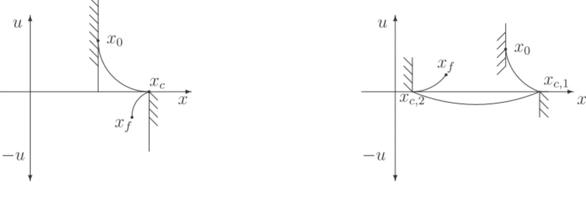
0 x0

1

A controllable state A state x0 is said to be controllable at time t0 if there exist a

control functionu.t /that steers the system into the origin in finite time; a statexf is said to be reachable if the system can be steered from the origin into xf in finite time. If the property holds for every statex and every t0 then the system will be called controllable (reachable). The system (2.1) is called observable on a finite intervalŒt0; T if any initial statex0 att0 can be determined from knowledge of the system outputy.t /and inputu.t /over the given interval.

0 xf

1

A reachable state

The controllability subspace is denoted by C, while the reachability subspace by R, respectively. For linear systems (complete) controllability and reachability are equivalent, i.e., the system is completely controllable if and only ifC DR DX.

Analogously U (O) denotes the unobservability (observability) subspace; Uis the set of all initial states that cannot be recognized from the output function. The system is observable if and only if U D0, i.e.,O DX.

A convenient way to study all solutions of a linear equation on the intervalŒ; , for all possible initial values simultaneously, is to introduce the corresponding transition matrix˚.; /¹:

x. /D˚.; /x. /C Z

˚.; t /B.t /u.t /dt D˚.; /.x0C Z

˚.; t /B.t /u.t /dt /:

Applying the time varying coordinate changez D˚.; t /xin the state space, the dynamic equation transforms into:

P

z D˚.; t /B.t /u.t /:

Thus in this new coordinate system controllability reduces to the solvability study of the equation:

z0 D Z

˚.; t /B.t /u.t /dt

for a suitable finite. If we denote by C the set of states controllable at thenC is a (closed) subspace, moreoverC1 C2 for1 < 2. Since the image space of the corresponding integral operator is finite dimensional, if the system is controllable there must be a finite² > 0N such that CN DRⁿ.

Hence, the controllability problem of an LTV system has been reduced to the question wether the finite rank operator L W L₂.Œ; ;N R^m/ ! Rⁿ defined as Lu D RN

˚.; t /B.t /u.t /dt is onto. These type of linear operators have a nice theory: it is immediate that the adjoint operator

1˚.t; t0/is nonsingular and˚.t; t0/DX.t /X ¹.t0/withX .t /P DA.t /X.t /; X.t0/DI; X.t /2Rⁿⁿ.

2Although it is essential for the reasoning, this statement is often missing from many of the available control text- books.

(17)

2 Motivation

L W Rⁿ ! L₂.Œ; ;N R^m/can be identified withLx D B.t /˚.; t /xand thatLis onto if and only ifLL> 0. So, the fundamental result (Kalman; 1960) concerning controllability of the LTV system (2.1) can be stated as the equivalence of the following statements:

Kalman’s Controllability Theorem: There exist a > 0such that K1. the controllability GrammianW .; /DR

˚.; s/B.s/B.s/˚.; s/dsis positive definite;

K2. there is no nonzero vectorp2Rⁿsuch thathp; ˚.; t /bi.t /i D0;fort 2Œ; ;andiD1; ; m:

It is a standard result (Silverman and Meadows; 1967) that one can derive a rank condition³that guarantees controllability while it does not involve integration and it can be obtained directly from the initial data matrices.A.t /; B.t //:

Silverman & Meadows Controllability Test: if (2.1)is analytic on an intervalJandt is an arbitrary fixed element ofJ;then the system is completely controllable on every nontrivial subinterval ofJif and only if

rank

B0.t / B1.t / Bk.t /

Dn; (2.5)

for some integerk;where

B0.t /WDB.t /; BiC1.t /WDA.t /Bi.t / d

dtBi.t /: (2.6)

If the analyticity condition is dropped, then the rank condition is only sufficient.

The problem is that it is hard to compute the rank of a time varying matrix, and we have no information about how to compute the controllability decomposition of the system⁴.

Kalman’s controllability result also reveals a structural property of linear systems: namely, by applying a suitable – in general time-varying – state transformation these systems decompose into a controllable an a purely uncontrollable part. To see this, suppose that there are at mostr vectors pi 2 X; hpi; ˚.; s/B.s/i D 0; s 2 Œ; . Chose them such that ˘˘ D I_r; where

˘ D Œ X. /pi. Considern r vectorsi 2 X orthogonal on pi;such that D I_{n r}; where D Œ X. /i. Then, the time varying matrix z D T x with T .t / D

˘

X ¹.t / transforms system (2.1) into thecontrollability decompositionform:

P

z1.t /D0 (2.7)

P

z2.t /DX ¹.t /B.t /u: (2.8) with the uncontrollable modez1.t /D˘X ¹.t /x.t /and with the completely controllable mode z2.t / D X ¹.t /x.t /. In other words, the reachable set isinvariant to the action of the controlled dynamics. The notion of invariance met in this context plays a central role in the investigations of geometric systems theory and it has been proven to be very useful in solving a series of control problems.

3For more details see the comments of Section A.2 of the Appendix.

4However, one can give a condition, when the system is surely uncontrollable: namely when the determinant of the matrix composed by the vectorsBi.t /vanishes.

(18)

2 Motivation

Linear time invariant (LTI) systems

In the framework of LTI theory the question of controllability can be decided by consulting the dimension of the reachability subspace, that can be computed easily from the initial data.A; B/of the problem, i.e.,

RD

n 1X

kD0

ImA^kB: (2.9)

Practically, the dimension of R is equal to the rank of the matrix whose columns are selected properly from those of the matricesA^kB, wherek D1; ; n 1:This condition is calledKalman rank condition.

The reachability set is a subspace and knowing this subspace one can decompose the system in a controllable and an uncontrollable part by using a state transformation that does not depend ont. Moreover, for LTI systems the different stabilizability properties are strictly related to controllability.

For practical reasons it would be very convenient to give – if it is possible – a characterization of the controllability property for a larger class of systems by using only matrix manipulations and to construct the controllability decomposition by using a time independent state transformation matrix.

2.2 Controllability of linear affine systems

For affine time dependencyA.t / D PN

iD1i.t /Ai the fundamental matrix can be given, at least locally, in terms of thecoordinates of second kind(Wei and Norman; 1964), i.e., the solutions of the Wei–Norman equation:

P

g.t /D. XK

iD1

e ¹^g¹ e ⁱ ¹^gⁱ ¹Ei i/ ¹.t /; g.0/D0: (2.10)

Here.t /DŒ1.t /; : : : ; N.t /^T andf OA1; : : : ;AOKgis a basis of the Lie-algebraL.A1; : : : ; AN/, the structure matrices i DŒ_i;j^l l;jD1;;K of the algebra are given byŒAOi;AOj DPK

lD1_i;j^l AOl

andEi i is the matrix with a single nonzero unitary entry at thei-th diagonal element.

Locally, the fundamental matrix is given by the expression:

˚.t / De^g¹^{.t /}ÂÔ¹e^g²^{.t /}ÂÔ² e^gⁿ^{.t /}ÂÔⁿ; (2.11) and generally it is not available in closed form.

Exploiting the affine structure and using the Peano–Baker formula for the transition matrix one can prove the following result:

(19)

2 Motivation

Lemma 1: For affine linear systems the points attainable from the origin are those from the subspaceR.A;B/

given by:

R.A;B/ Dspanf YJ

jD1

Aⁱ_l^j

jBkjJ 0; lj; k 2 f0; ; Ng; ij 2 f0; ; n 1gg; (2.12) i.e.,RR.A;B/.

Moreover, if one consider the finitely generated Lie-algebra L.A0; : : : ; AN/which contains the matrices A0; : : : ; AN;and a basisAO1; : : : ;AOKof this algebra, then

R.A;B/ D XN

lD0 n 1X

n1D0

: : : Xn 1

nKD0

Im.AOⁿ₁¹: : :AO_Kⁿ^KBl/:

A direct consequence of this fact is that if the inclusion RA;B Rⁿ is strict, i.e, ifRA;B is a proper subspace, then the system (2.1) cannot be completely controllable.

The main question is that under which condition is the reachability set equal to the Lie algebra, i.e., when we have R D RA;B. In what follows, if this property holds, then the system will be called c-excited. Characterization of this property by using only the initial data seems to be difficult. However, from conditionK2:of the Kalman’s controllability result, one has the following statement:

Proposition 1: A system is c-exciting if and only if the following implication holds: there exist a nonzero 2Rⁿsuch that

B.t /˚.t0; t / D0 for allt 2 Œt0; T implies that

RA;B˚.t0; t / D0 for allt 2 Œt0; T :

It is clear, that for c-excited systems controllability is guaranteed if the relationRA;B DRⁿ, i.e., themultivaraiable Kalman rank condition, holds. Moreover, if the rank condition does not hold, for this class of sytems one can construct the controllability decomposition by using a time independent state transformation matrix that depends only on the matrix Lie algebra.

Therefore it would be useful to give a condition that uses the original data only to decide wether a system is c-exciting or not. Unfortunately, such a condition has not been available yet.

In Szigeti (1992) a sufficient condition for for a system to be c-excited is given by the following property:

Szigeti, Controllability Test: The systemxP D A.t /xCBuwith affine time dependency is c–persistently excited onŒt0; T if from the equalities

BA_i₁ A_i_lA.t /˚.t0; t /pD0 (2.13) follows

BA_i₁ A_i_lA_j˚.t0; t /pD0; j D0; ; N; (2.14) wherepis a no nonzero vector inRⁿ:

(20)

2 Motivation

This property was characterized indirectly, in terms of the coordinates of second kind, i.e., the solutions of the Wei–Norman equation in Szigeti et al. (1995):

Szigeti, c-excitedness Test: Letibe smooth functions. If the components of the fundamental solutions of the linear affine differential equation are differential–algebraically independent, i. e., there is no non–trivial polynomial differential equation

P .g;g;P ; g^.q//D0;

then the multivariable Kalman rank condition is equivalent to the controllability of system.

c-excited systems versus linear independency

Let us consider systems with constant B and such that A.t / has an affine structure; then the fundamental matrixQ.t /can be written as

Q.t /D

n 1X

n1D0

: : : Xn 1

nKD0

AOⁿ₁¹: : :AO_Kⁿ^K n₁;;n_K.t /: (2.15)

Introducing the multi-index notationAOⁱ WD OAⁱ₁¹: : :AO_Kⁱ^K, withK WD f0; 1; n 1g^K andi WD .i1; ; iK/, let us choose a linearly independent set of matrices from the set f OAⁱji 2 Kg; say f OA^jjj2 j; j Kg. For the sake of simplicity, let us assume thatIis a member of this basis, i.e., one can impose the condition thatŒ'j.0/j2jis the first canonical unit vector. With these notations, one has

Q.t /DX

j2j

AO^j'j.t /: (2.16)

The systemf'_j. /jj2jgis not necessarily linearly independent and it can be obtained as the first column of the fundamental matrix associated to the equation

PQ

QD Q.t /;Q Q.0/Q DI; (2.17)

where.t /is a structure matrix⁵depending on the matrix Lie algebra and on the parameter functions.t /. Note, that from this derivation the systemf'j. /jj2 jgis not necessarily unique, but our choice satisfy (A.6).

Since the subspaceRA;B is exactly the image space of the matrix

R^A;B WDŒAOjB j2j; (2.18)

one can obtain the expression

W .; /DRA;B. Z

Œ '_j.s/ _j2jŒ '_j.s/ _j2jds/R_A_;_B:

5For details see the Appendix, Subsection A.1.

(21)

2 Motivation

It is clear that if the systemf'j. /jj2 jgis linearly independent thenrankW .; /DrankRA;B, i.e., the system is c-exciting.

Suppose now that rankRA;B D m, where m n, and let us consider the singular value decompositionRA;B DUS Vof this matrix. Then

rankW .; /DrankŒI_m0 .

Z

Œ'Q_j.s/ j2jŒ'Q_j.s/ _j2jds/ŒI_m0 ;

whereŒ'Qj.s/ j2J D VŒ 'j.s/ j2j. This set of functions can be chosen as the first column of the fundamental matrix associated to the equation:

˘P D .t /˘N ˘ .0/DV; (2.19) with.t /N D V.t /V. It follows that if the functionsf Q'0; ;'Qmgare linearly independent, thenrankW .; /DrankRA;B. Putting these facts together, one has the following result:

Proposition 2: The time varying system is c-excited if and only if the functionsf Q'0; ;'Qmgare linearly independent, wherem DrankR^A;B.

Remark 1: As an example, for LTI systems one has Q.t / D Pn 1

jD0A^j'j.t /. Suppose, that Aⁿ D Pn 1

kD0 ˛kA^k. Then, the matrixis given by

D 2 66 66 64

0 0 0 0 ˛0

1 0 0 0 ˛1

0 1 0 0 ˛2

:::

0 0 0 1 ˛n 1

3 77 77 75

;

and the systemf'j.t /jj D 0; ; n 1g is the first column of the fundamental matrix of the equation PQ

Q D Q;Q Q.0/Q D I. By an elementary argument one can show that these function are are always linearly independent, i.e., the LTI system is always c-excited, regardless to the matrixB.

For an affine LTV system if the functionsŒ _j.s/ _j2jare not linearly independent, the c-excitedness property depends onB.t /, too.

One can derive⁶an explicit expression, i.e., 'j.t /DX

n2N

˛ⁿ_jn.t /: (2.20)

between the functions Œ 'j.s/ j2j and the coordinate functions gi of the Wei–Norman formula.

This expression makes possible, in principle, the verification whether these functions are linear independent. However, the computational burden and the encountered numerical problems are so high that a practical application of the method for a real-sized application is out of the question.

To conclude this chapter a (negative) example is presented in order to demonstrate through a nonlinear dynamics, put into an affine qLPV form of (9.10), the importance of the c-excitedness property of the scheduling variables for controllability.

6For details see the Appendix, Subsection A.1.

(22)

2 Motivation

An illustrative example:

Let us consider the system

P

x1 Dx1x2Cx2 (2.21)

P x2 Du that can be rewritten asxP DA0CA1CBu, where

A0D 0 1

0 0

A1D 1 0

0 0

; B D 0

1

; and with Dx2.

SinceA0B D 1

0

one hasdimRA;B D2, i.e., the Kalman rank condition holds.

Applying the Silverman Meadows approach, one hasB0 DBandB1DA0B, i.e.,rankŒB0B1D 2, that shows that the system is controllable for any.t /:

Using the Wei–Normann theory, one hasŒA0; A1 D A0, i.e., ₀₁⁰ D 1; ₁₀⁰ D 1and the rest of the_ij^l D0:It follows that

1D

0 1 0 0

; 2 D 1 0

0 0

; i.e., e ¹^t D

1 t 0 1

; e ²^t D

e^t 0 0 1

: From

E11Ce ¹^g¹E22 D

1 g1

0 1

; it follows that the Wei–Normann equations are

P

g1Dg1C1 P

g2D:

The fundamental solution is given by˚.t /De ¹^A⁰e ²^A¹, i.e.,˚.t / D

e^g² g1

0 1

.

If the system is uncontrollable, according to the Kalman condition there should be a nonzero vector such thatB˚ .t / D0for allt, i.e., a numbermust exists such thate ^g²g1C D 0. But such a number does not exists⁷, hence the system should be controllable.

However, it is immediate thatx1 D 1is an uncontrollable manifold of system (2.21).

The reason why these tests fail relays in the fact that the uncontrollable manifold, i.e.,. 1; x2/ is not a subspace, while in the linear case the set of uncontrollable points is always a subspace.

If one shift the system from the equilibria point . 1; 0/;to .0; 0/, i.e., apply a (time-varying) change of coordinatesz1 D x1C1; z2 D x2, then one has the systemzP1 D z1z2; zP2 D u, withA./N D

0 0 0

;and Dz2 Dx2, that is clearly uncontrollable.

7Otherwise ^d.e ^g²g1/D0, i. e., gP2g1C Pg1D0; but the left hand side is1.

(23)

2 Motivation

2.3 Conclusions

One of the main motivation doing this "tour de force" in this introductory chapter along a classical topic of linear control theory was to illustrate that the controllability problem cannot be tackled in a mathematical completeness and rigor even for linear systems, if the system is time varying. The situation is even worse if the dynamics is actually nonlinear, but cast as a qLPV system. This stays in contrast to the familiar framework of LTI systems where the answer to the fundamental problem concerning controllability is very accessible and transparent. Filling the gap between these two extremities was one of the motivation backgrounds of my research.

The short review presented on the previous sections, however, reveals that the simplicity of the time invariant results might be regained in that of a splitting of the state space in a surely uncontrollable mode and a mode, that might be controllable. Controllability of this mode cannot be in- ferred, in general, only if some additional conditions on the parameters are fulfilled (c-excitedness).

Moreover, the simple example at the end of the chapter warn us on the inherent limitations of the approach when trying to extend it for nonlinear systems. It turns out, however, that for the class of linear switched systems (2.4), that despite of the linearity of the individual modes are true nonlinear systems, there always exists a c-exited switching sequence, which explains the effectiveness of the geometric (algebraic) treatment presented in the next chapter.

Concerning the (q)LPV systems (2.3) with affine parameter dependence the main issue is the problem of finding a time independent – and global – state transformation that splits the state space into modes that has specific properties – in these examples potentially controllable/uncontrollable modes. Concentrating on a rigorous proof of the controllability of the potentially uncontrollable mode is futile: not only due to the encountered mathematical difficulty of the computations but also due to the inherent uncertainty present in every practical model used in a nontrivial engineering application.

Affine (polytopic) LPV models considered in the thesis reflect the fact that the structure of the model (the system matrices) is known while the scheduling variables are often given by some ap- proximations or lookup–tables. Therefore trying to test wether they fulfill some differential polynomial relations, in order to check a c-exitedness property for controllability, is not reasonable. The most that can be supposed, in general, that they are linearly independent, a condition that will be exploited in the forthcoming chapters.

This fact motivates our desire in finding certain "robust" invariant subspaces that often provides acceptable (sufficient) conditions to obtain an engineering solution for a series of basic control problems. What we apparently miss in these constructions, i.e., the knowledge of controllability/observability, might cause problems at a different (higher) level of the design: namely, in obtaining stable controllers or filters. Lacking of a stable design might be a clear indication that our assumptions on the c-exitedness of the scheduling variables might not hold, or, more likely, our techniques to ensure stability are too conservative. Hence, a different approach should be used.

The proposed geometric framework based on parameter varying invariant subspaces provides an example for a strategy, in which giving up to get the complete mathematical solution of the problem but not sacrificing the mathematical correctness in following a more "rough" route to an acceptable result leads to a useful, engineering design.

(24)

Part I

Controllability

(25)

3 Linear switched systems

A switching system is composed of a family of different (smooth) dynamic modes such that the switching pattern gives continuous, piecewise smooth trajectories. We assume that one and only one mode is active at each time instant. During the last decade there has been a considerably interest in the analysis and synthesis of linear switched systems, intended as the simplest class of hybrid systems.

A lot of work has been done to address the fundamental questions of control theory – controllability, observability, stabilizability – that were reported in a series of papers, Liberzon and Agrachev (2001); Ge et al. (2001); Xie et al. (2002a); Cheng and Chen (2003); Lin and Antsaklis (2005b);

Sun et al. (2003) and monographs like Liberzon (2003); Sun and Ge (2005), just to list a few of them.

Controllability of switched systems has been investigated mostly for the case when arbitrary switching is possible (open–loop switching) and the objective is to design a proper switching sequence to ensure controllability or stability of (usually) piecewise linear systems, see Altafini (2002), Sun et al. (2003), Xie and Wang (2002), Yang (2002), or Sontag and Qiao (1999) for recurrent neural networks. Usually the input setUis assumed to be unconstrained, i.e.,U DR^m, however for certain systems, e.g., in process engineering applications where the inputs cannot be negative due to physical reasons, the sign constrained caseUDR^m

C is more relevant.

For LTI systems the controllability question was entirely solved. Moreover there is a controllability condition that describes both the unconstrained and constrained problems, Korobov (1980);

Frankowska et al. (1986). It turns out that a condition of the same type can be also formulated for switching systems. The elaboration of the solution to the controllability problem gives an opportunity to revise the main tools applied to the investigation of linear switched systems and to reveal facts and relations that remain hidden in previous works. In the elaboration of the topic advanced techniques like the geometric control theory of Jurdjevic (1997); Grasse and Sussmann (1990);

Agrachev and Sachkov (2004), nonsmooth analysis and differential inclusions of Aubin and Cellina (1984); Wolenski (1990); Dontchev and Lempio (1992); Smirnov (2002) met the more elementary techniques of Wonham (1985).