(2009) pp. 15–28
http://ami.ektf.hu
Approximation approach to performance evaluation of Proxy Cache Server systems
Tamás Bérczes
Department of Informatics Systems and Networks, University of Debrecen
Submitted 8 January 2009; Accepted 15 April 2009
Abstract
In this paper we treat a modification of the performance model of Proxy Cache Servers to a more powerful case when the inter-arrival times and the service times are generally distributed. First we describe the original Proxy Cache Server model where the arrival process is a Poisson process and the service times are supposed to be exponentially distributed random variables.
Then we calculate the basic performance parameters of the modified perfor- mance model using the well known Queueing Network Analysis (QNA) ap- proximation method. The accuracy of the new model is validated by means of a simulation study over an extended range of test cases.
Keywords: Queueing Network, Proxy Cache Server, Performance Models, GI/G/1 queue
1. Introduction
The Internet quickly became an essential and integral part of today’s life. How- ever, the booming use of the Web has caused congested networks and overloaded servers. So, the answer from the remote Web server to the client often takes a long time. Adding more network bandwidth is a very expensive solution. From the user’s point of view it does not matter whether the requested files are on the firm’s computer or on the other side of the world. The main problem is that the same object can be requested by other users at the same time. Because of this situation, identical copies of many files pass through the same network links, resulting in an increased response time. By preventing future transfer, we can cache information and documents that reduces the network bandwidth demand on the external net- work. In general, there are three types of caches that can be used in isolation or in a hierarchical fashion. Caching can be implemented at browser software [2]; the originating Web sites [3]; and the boundary between the local area network and the
15
Internet [4]. Browser cache are inefficient since they cache for only one user. Web server caches can improve performance, although the requested files must delivery through the Internet, increasing the response time. In this paper we investigate the third type. Requested documents can be delivered directly from the Web server or through a Proxy Cache Server (PCS). A PCS has the same functionality as a Web server when looked at from the client and the same functionality as a client when looked at from a Web server. The primary function of a PCS is to store documents close to the users to avoid retrieving the same document several times over the same connection. It has been suggested that, given the current state of technology, the greatest improvement in response time will come from installing a PCS at the boundary between the corporate LAN and the Internet.
In this paper, we present an extended version of the performance model of a PCS (see [5, 7]) using a more powerful case when inter-arrival times and the service times are generally distributed.
The organization of the paper is as follows. In Section 2, renewal-based para- metric decomposition models are reviewed (see [1, 10]). In Section 3 we introduce a modified version of the original performance model of Proxy Cache Server, where we include the repetition loop at the Proxy Server. A detailed description of the generalized model is given in Section 4. Section 5 is devoted to the validation of the numerical results of the approximation. The paper ends with Comments.
2. The GI/G/1 approximation
The GI/G/1 approximation described here is an example of a method using Parametric Decomposition (see [10]) where the individual queueing nodes are an- alyzed in isolation based on their respective input and output processes. In this model, the arrival process is a general (GI) arrival process characterised by a mean arrival rate and a squared coefficient of variation (SQV) of the inter-arrival time and the service time may have any general distribution. To use the approxima- tion, we need only to know the mean and the squared coefficient of variance of the inter-arrival times and the service times. In order to apply this method, we assume that the arrival process to a network node is renewal, so the arrival intervals are independent, identically distributed random variables. Immediate feedback, where a fraction of the output of a particular queue enters the queue once again, needs special treatment. Before the detailed analysis of the queueing network is done, the method first removes immediate feedback in a queue by suitably modifying its service time.
This model contains procedures required for modeling of the basic network op- erations of merging, departure and splitting, arising due to the common sharing of the resources and routing decisions in the network. Futhermore, the approximation provide performance measures (i.e. mean queue lengths, mean waiting times, etc.) for both per-queue and per-network.
The parameters required for the approximation: Arrival process: (λA - the mean arrival rate), (c2A - the SQV of the inter-arrival time) and service time (τS
- the mean service time), and (c2S - the SQV of the service time) at a considered node.
The approximation method that transforms the two parameters of the inter- nal flows for each of the three basic network operations and the removal of the immediate feedback, as given in [1], is described in the following:
1)Merging GI traffic flows: The superposed process of n individual GI flows, each characterized by λj and c2j (j = 1, . . . , n), as it enters the considered node is approximated by a GI traffic flow with parameters λA and c2S, representing the mean arrival rate and SQV of the inter-arrival time of the superposed flow, respectively. The mean arrival rate and the SQV of the inter-arrival time of the superposed flow is given by:
λA=
n
X
j=1
λj,
c2A=̟
n
X
j=1
λj
λA
c2j+ 1−̟,
with
̟= 1
1 + 4(1−ρ)2(ν−1),
ν= 1
Pn j=1
λ
j
λA
2, andρis the utilisation at the node, defined byρ=λAτS.
2) Departure flow from a queue: The departure flow from a queue is approx- imated as a GI traffic flow, characterized by λD and c2D, representing the mean departure rate and SQV of the inter-departure time of the departure flow, respec- tively. Under equilibrium conditions, the mean flow entering a queue is always equal to the mean flow existing the queue: λD=λA. The SQV of inter-departure time of the departure flow is given by:
c2D=ρ2c2S+ 1−ρ2 c2A
3)Splitting a GI flow Probabilistically: If a GI flow with parametersλandc2is split into n flows, each selected independently with probabilitypi, the parameters for the i-th flow will be given by:
λi =piλ, c2i =pic2+ (1−pi).
4)Removing immediate feedback: If the output traffic from a queue is fed back to this queue itself (Qi), so that the net arrival process is the sum of the external
arrivalsΛand the fed back portionpiiλi. The approach followed to eliminate this immediate feedback at the queue is to suitably adjust the service time at the queue and the SQV of service time. Assume that the original service parameters at the considered node are: τS,U- the mean service time, andc2S,U - the SQV of the service time. Removing the immediate feedback from that node we will get the modified service parameters:
τS,M = τS,U
1−pii
, c2S,M =pii+ (1−pii)c2S,U,
Wq,M = Wq,M
1−pii
.
This reconfigured queue without immediate feedback is used subsequently for solv- ing the queueing network.
5)Mean waiting time: If the considered node is a GI/G/1 queue, the following Kramer and Langenbach-Belz approximation is used (see [12]):
Wq =τS·ρ(c2A+c2D)β 2(1−ρ) with
βW eb=
(exp2(1
−ρ)(1−c2A)2 3ρ(c2A+c2D)
, forc2A<1, 1 forc2A>1.
3. The model of Proxy Cache Server
In this section we modified the original (M/M/1) performance model of Proxy Cache Server (see [5]). In this version of the performance model the Proxy Cache Server behaves like a Web server. So, if the size of the file that will pass through the server, is greater then the server’s output buffer it will start a looping process until the delivery of all file’s is completed (see [11, 6]).
Using Proxy Cache Server, if any information or file is requested to be down- loaded, first it is checked whether the document exists on the Proxy Cache Server or not. (We denote the probability of this existence byp). If the document can be found on the PCS then its copy is immediately transferred to the user. In the op- posite case the request will be sent to the remote Web server. After the requested document arrived back to the PCS then a copy of it is delivered to the user.
λ1 λ2
bandwith
Client network (1−qxc)λ′ λ′ PCS Server
Λ λ2 λ1
λ
PCS Lookup λ3
Server network bandwith
λ′3
(1−q)λ′3
λ′3 λ3 λ3 Λ
λ2
Web server Inilisation
Figure 1: Network model
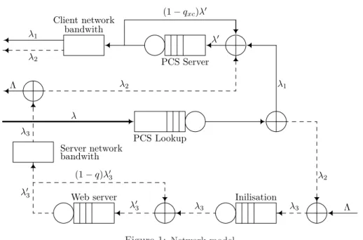
Figure 1 illustrates the path of a request in the original model (with feedback) starting from the user and finishing with the return of the answer to the user. The notations of the most important basic parameters used in this model are collected in Table 3.
In this section we assume that the requests of the PCS users arrive according to a Poisson process with rateλ, and the external requests arrive to the Web server according to a Poisson process with rateΛ, respectively.
The service rate of the Web server is given by:
µW eb= 1 YS+BRS
S
where Bsis the capacity of the output buffer,Ys is the static server time, andRs
is the dynamic server rate.
The service rate of the PCS is given by the equation:
µP CS = 1 Yxc+BRxc
xc
where Bxc is the capacity of the output buffer,Yxc is the static server time of the PCS, and Rs is the dynamic server rate of the PCS. The solid line in Figure 1 (λ1=pλ) represents the traffic when the requested file is available on the PCS and can be delivered directly to the user. Theλ2= (1−p)λtraffic depicted by dotted line, represents those requests which could not be served by the PCS, therefore these requests must be delivered from the remote Web server. λ3 = λ2+ Λ is the flow of the overall requests arriving to the remote Web server. First the λ3
traffic undergoes the process of initial handshaking to establish a one-time TCP connection (see [11, 7]). We denote byIsthis initial setup.
If the size of the requested file is greater then the Web server’s output buffer it will start a looping process until the delivery of all requested file’s is completed.
Let
q= min
1,Bs
F
be the probability that the desired file can be delivered at the first attempt. So λ′3 is the flow of the requests arriving at the Web service considering the looping process. According to the conditions of equilibrium and the flow balance theory of queueing networks
λ3=qλ′3
Also, the PCS have to be modeled by a queue whose output is redirected with probability1−qxc= min 1,BFxc
to its input, so λ=qxcλ′
where λ′ is the flow of the requests arriving to the PCS, considering the looping process.
Then we get the overall response time (see [5]):
Txc= 1
1
Ixc −(λ)+p
F Bxc
1
(Yxc+BxcRxc)−qλxc + F
Nc
+ (1−p)
1
1 Is −λ3
+
F Bs
1
(Ys+BsRs)−λq3
+F Ns
+
F Bxc
1
(Yxc+BxcRxc)−qλxc + F
Nc
.
(3.1)
4. The GI/G/1 model of Proxy Cache Server
In this section instead of M/M/1 queues we will use GI/G/1 queues using the approximation describe in Section 2.
λ1 λ2
bandwith Client network
λ
DPCS M2
λA
PCS Server S2
Λ λ2,R λ1
λ
PCS Lookup DLookup
λ3,DLookup
S1 Server network
bandwith
λ3,DWeb
DWeb
λ3,DInit
DInit M1
λ3 Λ
λ2
Web server Inilisation
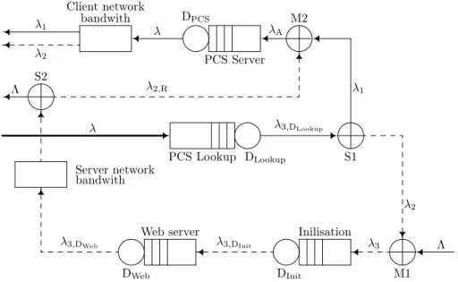
Figure 2: Modified Network model
The requests of the PCS users is assumed to be generalized inter-arrival (GI) process (see [10]) withλmean arrival rate and withc2λSQV of the inter-arrival time, and the external arrivals at the remote Web server are generalized inter-arrival process too with parametersΛandc2Λ.
The parameters of the queue PCS Lookup and the queue of the TCP initializa- tion (see Figure 2) areµLookup,c2Lookup andµInit,c2Init and the parameters of the Web and PCS servers areµW eb,c2W ebandµP CS,c2P CS where:
µLookup= 1 Ixc
, and
µInit= 1 IS
, µW eb= 1
YS+BRS
S
,
µP CS = 1 Yxc+BRxcxc
where Ixc is the lookup time of the PCS (in second) and Is is the TCP setup time. TheBsandBxcparameters are the capacity of the output buffer of the Web server and the PCS, Ys and Yxc are the static server times, andRs and Rxc are the dynamic server rates for the Web and Proxy servers (see [7]).
In the first step we removed the immediate feedbacks from the Web server and from the PCS, respectively. Figure 2 shows the modified model. After the removal
we have to modify the parameters of the corresponding servers:
µW eb,M =µW ebq, c2W eb,M= (1−q) +qc2W eb,
µP CS,M =µP CSqxc, c2P CS,M = (1−qxc) +qxcc2P CS.
In the model we have 2 superposition point (S1,S2), 2 merging point (M1,M2) and 4 separate queue where we have to recalculate the basic parameters. In S1 position the flow of the requests split in two flows with probabilitypand1−p.
The recalculated parameters of the departure flow after checked of the avail- ability of the required file are:
λD=λ,
c2DLookup =ρ2c2Lookup+ 1−ρ2 c2λ, where
ρ= λ µIxc
.
The solid line (λ1) represents those requests, which are available on the PCS and can be delivered directly to the user. Theλ2 traffic depicted by dotted line, repre- sents those requests which could not be served by the PCS, therefore these requests must be delivered from the remote Web server.
The parameters of the two flows are:
λ1=pλD, c21=pc2DLookup+ (1−p),
λ2= (1−p)λD, c22= (1−p)c2DLookup+p.
In M1 position the λ2 flow and the external requests are merging, and we get the λ3 flow with the parameters defined below:
λ3=λ2+ Λ, c23=w
λ2
λ3
c22+ Λ λ3
c2Λ
+ (1−w) where
w= 1
4(1−ρ)2(ν−1),
ν= 1
λ2
λ3
2
+
Λ λ3
2,
and
ρ= λ3
µInit
The parameters of the departure flow (λ3,DInit) after the TCP initialisation are:
λ3,DInit=λ3, c23,DInit =ρ2c2Init+ 1−ρ2
c23, where
ρ=λ3,DInit
µInit
.
The parameters of the departure flow (λ3,DW eb) from the Web server are:
λ3,DW eb =λ3, c23,DW eb =ρ2c2W eb,M+ 1−ρ2
c23,DInit, where
ρ= λ3
µW eb,M
.
Then in S2 position the λ3,DW eb flow splits into two parts. One part is the traffic of the external requests, with probability λΛ
2+Λ, and the second part is the flow (λ2,R) of the returning requests to the PCS. The parameters of theλ2,Rtraffic are:
λ2,R=λ2, c22,R= λ2
λ2+ Λc23,DW eb+
1− λ2
λ2+ Λ
In M2 position theλ1 traffic and theλ2,Rtraffic are merging intoλAtraffic which is described by parameters:
λA=λ1+λ2,R=λ1+λ2=λ, c2A=w
λ1
λc21+λ2
λc22,R
+ (1−w) where
w= 1
4(1−ρ)2(ν−1),
ν = 1
λ1
λ
2
+ λλ22, and
ρ= λ
µP CS,M
The overall response time can be calculated as follows (see [5, 11]):
Txc=TLookup+p
TP CS+ F Nc
+ (1−p)
TInit+TW eb+ F
Ns+TP CS+ F Nc
, where
TLookup=WLookup+ 1 µLookup
=
=
1
µLookupρLookup
c2λ+c2Lookup β
2 (1−ρlookup) + 1 µLookup
,
β =
exp
−
2(1−ρLookup)(1−c2λ)2
3ρLookup(c2λ+c2Lookup)
forc2λ<1
1 forc2λ>1
ρLookup= λ µLookup
and
TP CS=WP CS+ 1 µP CS,M
=
=
1
µP CS,Mρpcs c2A+c2pcs,M β 2 (1−ρpcs) + 1
µpcs,M
, where
β=
exp
−
2(1−ρpcs)(1−c2A)2
3ρpcs(c2A+c2pcs,M)
forc2A<1 1 forc2A>1
ρpcs= λA
µpcs,M
and
TInit=WInit+ 1 µInit
=
=
1
µInitρInit c23+c2Init βInit
2 (1−ρInit) + 1 µInit
, where
βInit=
exp
−
2(1−ρInit)(1−c23)2
3ρInit(c23+c2Init)
,forc23<1
1 forc23>1
ρInit= λ3
µInit
and
TW eb=WW eb+ 1 µW eb,M
=
=
1 µW eb,Mρweb
c2DInit+c2web,M βweb
2 (1−ρweb) + 1 µweb,M
,
βW eb=
exp
−
2(1−ρweb)(1−c2DInit)2
3ρweb
c2DInit+c2web,M
,forc2DInit <1 1 forc2DInit >1
ρweb= λ3
µweb,M
5. Numerical results
For the numerical explorations the corresponding parameters of Cheng and Bose [7] are used. The value of the other parameters for numerical calculations are:
Is=Ixc = 0.004seconds, Bs =Bxc = 2000bytes, Ys=Yxc = 0.000016 seconds, Rs=Rxc= 1250Mbyte/s,Ns= 1544Kbit/s, andNc= 128Kbit/s. These values are chosen to conform to the performance characteristics of Web servers in [9].
For validating the approximation, we wrote a simulation program in Microsoft Visual Basic 2005 under .NET framework 2.0. It was run on a PC with a T2300 Intel processor (1.66 GHz) with 2 GB RAM. First we validated the simulation pro- gram using exponential distributions. For validation we calculated the analytical results of the overall response time given by Eq(3.1) and compared to the simu- lation results. In Table 1, we can see that the corresponding mean of the total response times are very close to each other; they are the same at least up to the 4th decimal digit.
For the validation of the approximation method we used the following dis- tributions (see [8]). In case 0 < cX < 1 we use an Ek−1,k distribution, where
1
k 6k < k1
−1. In this case the approximating Ek−1,k distribution is with proba- bility p (resp. 1−p) the sum of k−1 (resp. k) independent exponentials with common mean 1µ. Choosing
p= 1 1 +c2X
kc2X− k 1 +c2X
−k2c2X1/2
and µ= k−p E(X) theEk−1,k distribution matchesE(X)andcX.
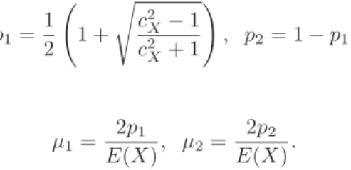
In casecX >1 we fits aH2(p1;p2;µ1;µ2)hyper-exponential distribution with balanced mean (see [8]):
p1
µ1
= p2
µ2
So the parameters of thisH2distributions are:
p1=1 2 1 +
s c2X−1 c2X+ 1
!
, p2= 1−p1,
and
µ1= 2p1
E(X), µ2= 2p2
E(X).
For the easier understanding we used for all queues the same SQV rate. In Table 2, we show the results of the simulations and approximations with various parameters.
Parameters Analytical result Simulation result Approximation Difference λ= 20,Λ = 100 0.425793 0.425706 0.425793 0.000087 λ= 80,Λ = 100 0.430135 0.430136 0.430135 0.000001
Table 1: Exponential distribution
Arrival intensity SQV Simulation result Approx. result Difference
0.1 0.423084 0.423129 0.000045
λ= 20 0.8 0.425127 0.425189 0.000062
Λ = 100 1.2 0.423042 0.426328 0.003286
1.8 0.421744 0.427979 0.006235
0.1 0.423591 0.423974 0.000383
λ= 80 0.8 0.428624 0.428725 0.000101
Λ = 100 1.2 0.425821 0.431507 0.005686
1.8 0.424049 0.435869 0.011820
Table 2: Approximation
6. Comments
In this paper we modified the performance model of Proxy Cache Server to a more powerful case when the arrival processes is a GI process and the service times may have any general distribution. To obtain the overall response time we used the QNA approximation method, which was validated by simulation. As we can see in Table 2, when theSQV <1the overall response time obtained by approximation is very close to response time obtained by simulation; they are the same at least up to the 3–4th decimal digit. In case when the SQV > 1 the response times are the same only to 2–3th decimal digit. We can see, when the SQV = 1.2 the difference between the response times are 0.005686, and when theSQV = 1.8the difference between the response times is greater (0.01182). So, using greater SQV the approximation error is greater.
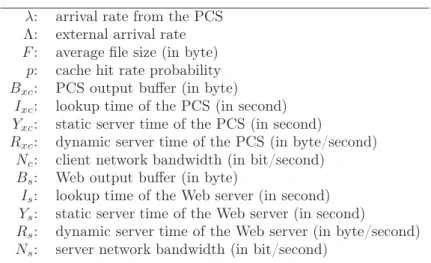
Table 3: Notations λ: arrival rate from the PCS
Λ: external arrival rate F: average file size (in byte)
p: cache hit rate probability Bxc: PCS output buffer (in byte)
Ixc: lookup time of the PCS (in second) Yxc: static server time of the PCS (in second)
Rxc: dynamic server time of the PCS (in byte/second) Nc: client network bandwidth (in bit/second)
Bs: Web output buffer (in byte)
Is: lookup time of the Web server (in second) Ys: static server time of the Web server (in second)
Rs: dynamic server time of the Web server (in byte/second) Ns: server network bandwidth (in bit/second)
References
[1] Atov I., QNA Inverse Model for Capacity Provisioning in Delay Constrained IP Networks. Centre for Advanced Internet Architectures. Technical Report 040611A Swinburne University of Technology Melbourne, Australia, (2004).
[2] Aggarwal, C.,Wolf, J.L.andYu, P.S., Caching on the World Wide Web.IEEE Transactions on Knowledge and Data Engineering, 11 (1999) 94–107.
[3] Almeida, V.A.F.,de Almeida, J.M. andMurta, C.S. Performance analysis of a WWW server.Proceedings of the 22nd International Conference for the Resource Management and Performance Evaluation of Enterprise Computing Systems, San Diego, USA, December 8. 13 (1996).
[4] Arlitt, M.A.andWilliamson, C.L.Internet Web servers: workload characteri- zation and performance implications. IEEErACM Transactions on Networking, 5 (1997), 631–645.
[5] Berczes, T.andSztrik, J., Performance Modeling of Proxy Cache Servers.Journal of Universal Computer Science., 12 (2006) 1139–1153.
[6] Berczes, T.,Guta, G.,Kusper, G.,Schreiner, W.andSztrik, J., Analyzing Web Server Performance Models with the Probabilistic Model Checker PRISM.Tech- nical report no. 08-17 in RISC Report Series, University of Linz, Austria. November 2008.
[7] Bose, I. and Cheng, H.K., Performance models of a firms proxy cache server.
Decision Support Systems and Electronic Commerce., 29 (2000) 45–57.
[8] Henk C. TijmsStochastic Modelling and Analysis. A computational approuch.John Wiley & Sons, Inc. New York, (1986).
[9] Menasce, D.A.and Almeida, V.A.F.,Capacity Planning for Web Performance:
Metric, Models, and Methods.Prentice Hall., (1998).
[10] Sanjay K. BoseAn introduction to queueing systems. Kluwer Academic/Plenum Publishers, New York, (2002).
[11] Slothouber L.P., A model of Web server performance. 5th International World Wide Web Conference, Paris, Farnce., (1996).
[12] Whitt, W., The Queueing Network Analyzer.Bell System Technical Journal., Vol.
62, No. 9 (1983) 2799–2815.
Tamás Bérczes
Department of Informatics Systems and Networks University of Debrecen
P.O. Box 12 H-4010 Debrecen Hungary
e-mail: berczes.tamas@inf.unideb.hu