Optimization of coefficients of lists of polynomials by evolutionary algorithms
J. Rafael Sendra
a, Stephan M. Winkler
baUniversity of Alcalá, Department of Physic and Mathematics Rafael.Sendra@uah.es
bUpper Austria University of Applied Sciences, Heuristic and Evolutionary Algorithms Laboratory
Stephan.Winkler@fh-hagenberg.at
Submitted July 30, 2014 — Accepted December 12, 2014
Abstract
We here discuss the optimization of coefficients of lists of polynomials using evolutionary computation. The given polynomials have 5 variables, namelyt,a1,a2,a3,a4, and integer coefficients. The goal is to find integer valuesαi, with i∈ {1,2,3,4}, substituting ai such that, after crossing out the gcd (greatest common divisor) of all coefficients of the polynomials, the resulting integers are minimized in absolute value. Evolution strategies, a special class of heuristic, evolutionary algorithms, are here used for solving this problem. In this paper we describe this approach in detail and analyze test results achieved for two benchmark problem instances; we also show a visual analysis of the fitness landscapes of these problem instances.
Keywords: Optimization of parametrizations, symbolic computation, evolu- tionary computation, evolution strategies.
MSC:65K10, 68T05, 68W30
1. Problem statement
In this section, trying to avoid as much as possible mathematical technicalities, we describe the problem, and we explain its interest in the field of mathematics.
http://ami.ektf.hu
177
The problem statement. We are given a list with infinitely many (at least 3) non-constant polynomials (L = [p1;p2;. . .;pn]). These polynomials have 5 vari- ables, namely t, a1, a2, a3, a4, and integer coefficients. The problem consists in finding integer valuesα1, α2,α3, andα4 fora1,a2,a3, anda4 such that:
1. α1α4−α2α36= 0
2. We substitute a1=α1,a2=α2,a3=α3,a4=α4, inL. This yieldsL0(α), a list of polynomials with one variable, namelyt, and integer coefficients. We cross out the greatest common divisor (gcd) of all non-zero coefficients of the polynomials inL0(α)to get a new listL00(α).
The goal is to find that substitutionai=αi,i∈ {1,2,3,4}, so that the maximum of the absolute values of all the coefficients of all polynomials inL00(α)is minimum.
An illustrating example. We consider the list with three polynomials L = [p1;p2;p3] where
p1(t) = 13923t2a12+ 5474t2a1a3−1904t2a32+ 27846ta1a2+ 5474ta1a4
+ 5474ta2a3−3808ta3a4+ 13923a22+ 5474a2a4−1904a42
p2(t) = 7564t2a12
−10298t2a1a3−990t2a32+ 15128ta1a2−10298ta1a4
−10298ta2a3−1980ta3a4+ 7564a22
−10298a2a4−990a42
p3(t) = 15845t2a12
−106t2a1a3+ 2146t2a32+ 31690ta1a2−106ta1a4
−106ta2a3+ 4292ta3a4+ 15845a22
−106a2a4+ 2146a42
If we substitutea1= 1, a2= 1, a3= 1, a4= 1we get
L0(α) = [17493t2+34986t+17493;−3724t2−7448t−3724; 17885t2+35770t+17885]
Sincegcd(17493,34986,17493,−3724,−7448,−3724,17885,35770,17885) = 49, one getsL00(α) = 1/49L0(α), that is
L00(α) = [357t2+ 714t+ 357;−76t2−152t−76; 365t2+ 730t+ 365]
and the maximum, in absolute value, is 730. However, if we take a1 = 45, a2 = 11, a3= 31, a4=−122 the new list is
L0(α) = [34000561t2−34000561; 68001122t; 34000561t2+ 34000561].
The corresponding gcd is now34000561. Therefore
L00(α) = 1
34000561L0(α) = [t2−1; 2t;t2+ 1]
whose maximum, in absolute value, is 2.
The mathematical origin of the problem. This optimization question, we are dealing with, comes from a central problem in the field of the symbolic com- putation of algebraic curves (see [6] for further details), appears in many compu- tational aspects of the practical applications of curves and is, to our knowledge, not solved. Let us first motivate the problem: In many practical applications, such as in computed aided geometric design, in physics, etc., one deals with parametric representations of a curve. For instance, if we have to compute a line integral along an arc of the curve of equationy3=x2, we might use the parametric representation x=t3, y =t2 of the curve. In general a rational parametrization of a curve, say for simplicity planar, is a nonconstant pair
p1(t) q(t),p2(t)
q(t)
where p1, p2, q are polynomials in the variable t. The difficulty here is the fol- lowing: If we replace t by a polynomial or by a rational function, then we get another parametrization of the same object; for instance, in the example above, (1000t3,100t2) and ((t2 + 1)3,(t2 + 1)2) are also parametrizations of y3 = x2. Thus, we have infinitely many possibilities, but some parametrizations are more complicated and increase the computational time when using them. The question is how to choose the simplest parametrization. Achieving an optimal degree in the polynomials is solved by means of symbolic deterministic algorithms (see [6]). How- ever, the question of determining a parametrization with the smallest (in absolute value) integer coefficients is open. Here, in this paper, we show how to approach the problem by means of evolutionary algorithms.
In order to translate the original parametrization problem into the the prob- lem stated above, we use Lüroth’s theorem that establishes how all parametriza- tions, with optimal degree, are related. More precisely, if P(t) = (PQ(t)1(t),PQ(t)2(t)) is a parametrization with optimal degree and integer coefficients, then all the other parametrizations with optimal degree and integer coefficients are of the form
P
a1t+a2
a3t+a4
=
P1
a1t+a2
a3t+a4
Q
a1t+a2
a3t+a4
, P2
a1t+a2
a3t+a4
Q
a1t+a2
a3t+a4
,
wherea1, a2, a3, a4are integers such thata1a4−a2a36= 0. Simplifying this expres- sion, we get the three polynomials in the variables t, a1, a2, a3, a4.
Revisiting the illustrating problem. We are given the parametrization
P(t) =
13923t2+ 5474t−1904
15845t2−106t+ 2146,7564t2−10298t−990 15845t2−106t+ 2146
Performing the formal substitutiont= aa13t+at+a24, simplifying expressions and collect- ing numerators and denominators in a list we get the listL= [p1;p2;p3]of the three
polynomials shown above. Now, after takinga1= 45, a2= 11, a3= 31, a4=−122, we get the parametrization
P
45t+ 11 31t−122
=
t2−1 t2+ 1, 2t
t2+ 1
.
The parametrization in this example corresponds to the unit circlex2+y2= 1.
2. Parameter optimization by evolutionary algorithms
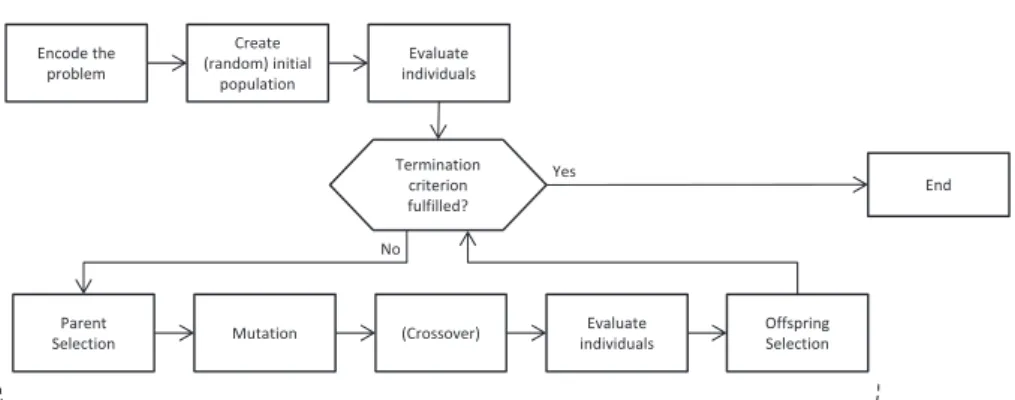
Evolution strategies (ES; [4], [5]), beside genetic algorithms (GA; [2], [1]) the second major representative of evolutionary computation, are here used for optimizing α1, . . . , α4. ES are population based, i.e., each optimization process works with a population of potential solution candidates that are initially created randomly and then iteratively optimized. In each generation, new solution candidates are generated by randomly selecting parent individuals and forming new individuals applying mutation and (optionally) crossover operators; λchildren are produced byµparent individuals.
By offspring selection, the best children are chosen and become the parents of the next generation. Typically, parent selection in ES is performed randomly with no regard to fitness; survival in ESs simply saves theµ best individuals, which is only based on the relative ordering of their fitness values. Basically, there are two selection strategies for ESs:
• The (µ, λ)-strategy (“comma selection”): µ parents produce λchildren; the bestµchildren are selected and form the next generation’s parents.
• The (µ+λ)-strategy (“plus selection”): µparents produceλoffspring; parents and children form a pool of potential new parents, and the bestµindividuals are selected from this pool to become the next generation’s parents.
Thus, the main driving forces of optimization in ESs are offspring selection and mutation. For the optimization of vectors of real values, mutation is usually implemented as additive Gaussian perturbation with zero mean or multiplicative Gaussian perturbation with mean 1.0. Mutation strength control [4] is based on the quotient of the number of the successful mutants (i.e., those that are better than their parents): If this quotient is greater than 1/5, then the mutation variance is to be increased; if the quotient is less than 1/5, the mutation variance should be reduced.
Encode the problem
Create (random)initial
population
Evaluate individuals
Evaluate individuals Parent
Selection Mutation (Crossover) Offspring
Selection
End Termination
criterion fulfilled?
Createnew generation Yes
No
Figure 1: The main workflow of an evolution strategy
3. Test series
3.1. Problem instances
We have used the following two test instances:
• The example (Ex1) introduced in Section 1
• The second example (Ex2) is defined asL2 = [p1;p2;p3]with
p1= 1685t2a12+ 2252t2a1a3+ 769t2a32+ 3370ta1a2+ 2252ta1a4
+ 2252ta2a3+ 1538ta3a4+ 1685a22+ 2252a2a4+ 769a42
p2=−627t2a12−1148t2a1a3−481t2a32
−1254ta1a2−1148ta1a4
−1148ta2a3−962ta3a4−627a22
−1148a2a4−481a42
p3= 2467t2a12+ 3235t2a1a3+ 1069t2a32+ 4934ta1a2+ 3235ta1a4
+ 3235ta2a3+ 2138ta3a4+ 2467a22+ 3235a2a4+ 1069a42
For this example, taking α1 =−25, α2 = 12, α3 = 34, α4 =−23(note that α1α4−α2α3= 1676= 0) we get
L0= [27889t2+ 27889; 27889t2−27889; 27889t2+ 27889t+ 27889].
The gcd is 27899 andL00= [t2+ 1;t2−1;t2+t+ 1]and the maximum of the absolute values is 1, which is clearly optimal.
3.2. Algorithm configurations
The following 10 algorithm variants have been used for solving the problems defined in the previous section:
Population Number of Selection size (µ) children (λ) mechanism
Settings 1 100 1,000 comma
Settings 2 100 10,000 comma
Settings 3 100 1,000 plus
Settings 4 100 10,000 plus
Settings 5 1,000 10,000 comma
Settings 6 1,000 100,000 comma
Settings 7 1,000 10,000 plus
Settings 8 1,000 100,000 plus
Settings 9 10,000 100,000 comma
Settings 10 10,000 100,000 plus
Table 1: Algorithm parameter settings used for solving the here discussed coefficients optimization problem.
The range of values for initial solution candidates was set to ±200. For cre- ating offspring we have used multiplicative mutation: The average value of the multiplication factors µ was set to 1.0, the standard deviation σ was initially set to 1.0 and according to the1/5 success rule updated after each generation (with multiplicative factor / divisor 0.9).
3.3. Results
We have executed ES test series using all parameter configurations defined previ- ously; each algorithm configuration was executed 5 times independently, and for guaranteeing a fair comparison of results the maximum number of evaluations used as termination criterion was set to 1,000,000. Thus, the number of generations ex- ecuted was not equal for all test configurations.
The results achieved in these test series are summarized in Table 2.
We see that the success rate for small populations is very low, when using bigger populations (with size 1,000 or 10,000) the results are significantly better; when using populations of size 1,000, then significantly better results are achieved using higher selection pressure, i.e. selecting the 1,000 best out of 100,000 offspring each generation.
Problem Ex1 seems to be harder for the algorithm than Ex2. For Ex1 the algorithm was able to find the optimal solution at least once using settings 8 and 10; forEx2the algorithm was successful in finding the optimum in 4 or 5 out of 5 runs using the settings 6, 8, 9, and 10.
Problem instanceEx1 Problem instanceEx2
Settings 1 4807.4 483.6
Settings 2 1270.6 402.2
Settings 3 2136.6 671.0
Settings 4 438.2 3.8
Settings 5 854.4 110.6
Settings 6 160.0 1.0
Settings 7 120.4 21.2
Settings 8 58.2 1.2
Settings 9 230.8 1.4
Settings 10 35.4 1.6
Table 2: Test results. For each algorithm configuration we give the average result qualities achieved for problem instancesEx1and
Ex2.
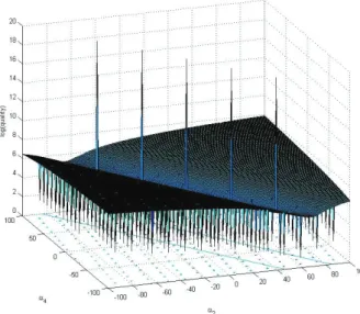
Fitness Landscape analysis [3] methods can be used for estimating an optimiza- tion problem’s hardness. As we see in Figures 2 and 3, the fitness landscape of the here used problem instances Ex1 and Ex2 are very rugged, which makes it very hard for optimization algorithms to find optimal solutions.
Figure 2: Fitness landscape analysis for example Ex1. We have created 40,000 solution candidates for Ex1 that are arranged on the x-y-plane; the optimal solution discussed in Section 1 (a1 = 45, a2 = 11, a3 = 31, a4 =−122) is positioned at (1,1), and at all other cells are assigned solution candidates that are produced by mutating one of their neighbors (using σ = 1.0). On thez-axis we draw the fitness of the so created solution candidates for Ex1.
We see high fluctuations of the fitness values which indicates that fitness values of neighboring solutions vary significantly.
Figure 3: Fitness landscape analysis for exampleEx2. All possible solution candidates for the here used problem with α1 andα3 set optimally (α1=−25,α3=−34) are created, their fitness is drawn on thez-axis. We see that even when setting two of four parameters
optimally, the resulting fitness landscape is very rugged.
4. Conclusion, outlook
Future work will concentrate on the improvement of mutation and selection opera- tors for this problem class in order to solve problem instances involving significantly bigger coefficients. Additionally, we are working on strategies to decrease the search space. We are also working on the integration of the here discussed class of prob- lems in HeuristicLab [7], a framework for heuristic and evolutionary algorithms that is developed by members of the Heuristic and Evolutionary Algorithms Laboratory (HEAL).
Acknowledgements. The authors thank Franz Winkler at the Research Insti- tute for Symbolic Computation, Johannes Kepler University Linz, for his advice.
R. Sendra is partially supported by the Spanish Ministerio de Economía y Competi- tividad under the project MTM2011-25816-C02-01 and is a member of the Research Group ASYNACS (Ref. CCEE2011/R34). The authors also thanks members of the Heuristic and Evolutionary Algorithms Laboratory as well as of the Bioinfor- matics Research Group, University of Applied Sciences Upper Austria, for their comments.
References
[1] M. Affenzeller, S. M. Winkler, S. Wagner, and A. Beham. Genetic Algorithms and Genetic Programming - Modern Concepts and Practical Applications. Chapman &
Hall / CRC, 2009.
[2] J. H. Holland. Adaption in Natural and Artifical Systems. University of Michigan Press, 1975.
[3] E. Pitzer.Applied Fitness Landscape Analysis. PhD thesis, Institute for Formal Models and Verification, Johannes Kepler University Linz, 2013.
[4] I. Rechenberg. Evolutionsstrategie. Friedrich Frommann Verlag, 1973.
[5] H.-P. Schwefel. Numerische Optimierung von Computer-Modellen mittels der Evolu- tionsstrategie. Birkhäuser Verlag, Basel, Switzerland, 1994.
[6] J. R. Sendra, F. Winkler, and S. Perez-Díaz. Rational Algebraic Curves: A Com- puter Algebra Approach. Algorithms and Computation in Mathematics. Volume 22.
Springer-Verlag Heidelberg, 2007.
[7] S. Wagner, G. Kronberger, A. Beham, M. Kommenda, A. Scheibenpflug, E. Pitzer, S. Vonolfen, M. Kofler, S. Winkler, V. Dorfer, and M. Affenzeller. Advanced Meth- ods and Applications in Computational Intelligence, volume 6 ofTopics in Intelligent Engineering and Informatics, chapter Architecture and Design of the HeuristicLab Optimization Environment, pages 197–261. Springer, 2014.