FUZZY RULE BASE IDENTIFICATION USING AN INCREMENTAL APPROACH
Zsolt Csaba Johanyák*
Department of Information Technology, GAMF Faculty of Engineering and Computer Science, John von Neumann University, Hungary
https://doi.org/10.47833/2021.2.CSV.004
Keywords:
fuzzy logic sparse rule base rule interpolation RBE-PSO Article history:
Received 8 September 2021 Revised 15 September 2021 Accepted 16 September 2021
Abstract
A sparse fuzzy rule base provides low complexity and low memory requirements for the fuzzy system. Automatic fuzzy model generation from sample data involves two main tasks. These are structure determination and parameter identification. In this paper, we present a new approach that initially generates two rules, then gradually adds new rules to the rule base, and then finds the quasi-optimal values of the parameters using particle swarm optimization.
1 Introduction
One of the most important steps in identifying a fuzzy model is to create a rule base. Often there is not enough expertise and experience to define the rules directly, but one can access a sample data set that shows, through specific cases, what output values are expected in case of some input value combinations. Based on these, one can automatically generate the rule base using a properly selected algorithm. Most well-known methods create a completely covering rule base, which can lead to an explosion of rule numbers for a large number of dimensions and a large number of sets per dimension.
The RBE-PSO (rule base extension with particle swarm optimization) method ensures a trade- off between the demand on approximation capability of the fuzzy system and the demand on low complexity of the rule base by generating a sparse rule base. It follows the concept of rule base extension [7][6] and identifies the parameters of the fuzzy system using particle swarm optimization method.
The rest of this paper is organized as follows. Section 2 presents the applicable membership function parameterization approaches. Section 3 introduces the new method after reviewing the concepts of sparse rule bases and rule base extension. Section 4 presents some experimental results applying RBE-PSO and the conclusions are drawn in section 5.
2 Parameterization
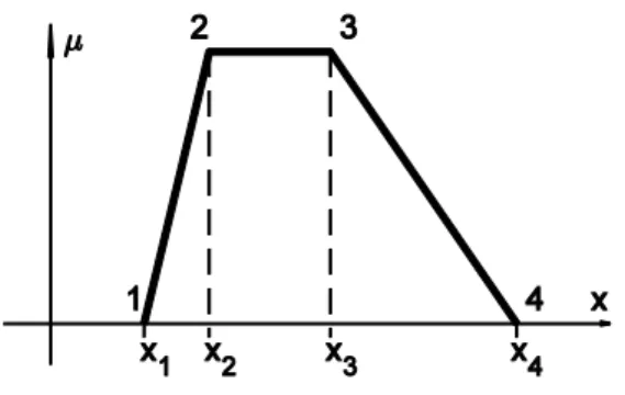
Each membership function can be described by a smaller or larger number of parameters depending on the shape type. The piece-wise linear membership functions can be described easily by the position of the break-points. For example in case of a singleton the parameter is the element of the universe of discourse whose membership value is greater than zero; or in case of a triangle shaped normal fuzzy set (e.g. Fig. 1) the parameters are the abscissa values of the three vertices.
Figure 1. Parameterization of a triangle shaped membership function
The number of the parameters determines the number of variables whose values are changed in course of the fuzzy model identification, which has a strong effect on the time need of the process.
In several cases one might use uniform shaped fuzzy sets in order to reduce the time demand. Thus only one parameter has to be adjusted in case of each linguistic term. This parameter is the position of the set described by the reference point. Usual choices for this task are abscissa values corresponding to the centre of the core (RPcc, e.g. [1][2][5]), the centre of gravity (RPgc, e.g.[4]) and the centre of the support (RPsc, e.g. [2]). In case of trapezoid shaped membership functions the respective reference points are calculated as follows.
𝑅𝑃𝑐𝑐 =𝑥3−𝑥2
2 (1)
𝑅𝑃𝑔𝑐= 𝑥1+2(𝑥3−𝑥2)(𝑥2−𝑥1)+(𝑥3−𝑥2)2+(𝑥2−𝑥1)(𝑥4−𝑥1)+(𝑥3−𝑥2)(𝑥4−𝑥1)+(𝑥4−𝑥1)2
3(𝑥3−𝑥2+𝑥4−𝑥1) (2)
𝑅𝑃𝑠𝑐 =𝑥4−𝑥1
2 (3)
Although the application of the uniform shaped sets reduces the time consumption of the tuning and preserves the good interpretability of the fuzzy rules it also can have a negative side effect by reducing the performance of the fuzzy system. Thus the selection of the parameterization is a trade- off between the performance of the system and the cost of the model identification.
3 Model identification from numerical sample data
The determination of the parameters of a fuzzy model usually starts with the identification of the input and output linguistic variables, determination of the lower or upper bounds of each dimension of the input and output universes of discourse, statistical analysis of the data regarding the relevance of the input variables excluding the non-relevant ones in order to reduce the complexity of the system. Next, an initial rule base is generated from the sample data, which is later refined in course on an iterative process employing an arbitrary search method. In the following two subsections some key ideas related to sparse rule bases and the inference process are going to be recalled followed by the presentation of the proposed approach.
3.1 Sparse rule base
The rule base of a fuzzy system can be considered dense (covering) or sparse (non-covering) (see Fig. 2) depending on the ε coverage level of the input space by rule antecedents, which is defined by the formula
,
0,1,, ,
max min
max
arg 1 1 , *
i i
i j i n
j N i
X A
A A t
c i
(4)
where Xi is the ith dimension of the antecedent space, 𝐴𝑖∗ is the fuzzy set describing the observation in the ith antecedent dimension, 𝐴𝑖,𝑗 is the jth linguistic term of the ith antecedent dimension, t is an arbitrary t-norm, ni is the number of the linguistic terms of the ith antecedent dimension, N is the number of the antecedent dimensions, and argmax(.) calculates the ε value for which the expression in the parentheses takes its maximum. If c> ε0 the rule base is called ε0 covering (dense) otherwise it is considered sparse.
Fig. 2 Sparse antecedent space
If there is no demand on an ε>0 value the rule base is considered sparse when there is at least one possible input value for which the rule base does not contain an applicable rule.
3.2 Fuzzy inference in sparse rule bases
Fuzzy systems applying sparse rule bases have to use approximate inference techniques that can cope with the lack on rules in some regions of the input space. For this task the most used techniques are the fuzzy rule interpolation based ones. They form two main groups based on the key ideas they are using.
The members of the first group, the so called one-step methods determine the conclusion directly from the observation taking into consideration two or more existent rules of the rule base.
The methods KH [14], FIVE [10], IMUL [16], IRG [2], and Kovács’s method [9] belong to this category.
The members of the second group first produce a new rule in the position of the observation using rule interpolation and next, they determine the conclusion by firing the interpolated rule. Here belong for example the methods GM [1], IGRV [4], and VLESFRI [5].
3.3 RBE-PSO
The rule base extension using particle swarm optimization (RBE-PSO) method aims the generation of a fuzzy rule base from numerical sample data. The data consist of known input and output value pairs. The input could be one- or multidimensional, while the output has to be one- dimensional. In case of a multidimensional output a separate rule base can be generated for each output dimension.
The basic idea of the Rule Base Extension (RBE) [7][6] is that one creates first an initial rule base and next, one starts an iterative tuning process when beside the adjustment of the values of the known sets’ parameters new linguistic terms and rules are introduced into the rule base.
The initial rule base contains only two rules, one describing a maximum point of the output and one describing a minimum point of the output. First one seeks the two extreme output values and a representative data point for each of them. If several data points correspond to an extreme value, one should select the one that is closer to an endpoint of the input domain.
The reference points of the antecedent sets of the first rule will be identical with the
by the default set shape, which is a characteristic feature of the partition. The antecedent and consequent linguistic terms of the second rule are determined in a similar way taking into consideration the maximum point. At this point the system contains two linguistic terms in each dimension.
Having the first two rules determined, next a parameter identification process is started, which iteratively adjusts the values of the linguistic terms’ parameters. The details of the applied algorithm are presented in the next section. If the improvement velocity of the fuzzy systems’ performance index falls below a specified threshold or even stops after an iteration cycle a new rule is generated.
It is because the system tuning reached a local optimum of the performance indicator and the performance cannot improve further by the applied parameter identification algorithm. The new rule introduces additional tuning possibilities. However, in some cases the performance will deteriorate temporarily after the insertion of the new rule into the rule base.
In order to create the new rule, one seeks for the calculated data point, which is the most differing one from its corresponding training point. The input and output values of this training point will be the reference points of the antecedent and consequent sets of the new rule. The shapes of the new linguistic terms are determined using the default shape types of the corresponding partition.
Further on, the last two steps (parameter adjustment and new rule creation) are repeated until the specified iteration number has been reached, or the value of performance index overcomes a prescribed threshold.
3.4 Parameter identification using Particle Swarm Optimization
The parameter identification/adjustment aims the determination of quasi-optimal values for the parameters of the fuzzy sets. In this research, the well-known Particle Swarm Optimization (PSO) [8] was employed for the task. In PSO terminology, a vector containing a set of the actual values of the parameters is called a particle. The search for the optimal values of these parameters is an iterative process where in course of each iteration a set of candidate solutions (particles) are considered, evaluated, and moved across the parameter/search space exploring it in some discrete points. The current location of a particle is described by its position vector in the search space, while in each iteration the new position is calculated by the help of the so called velocity vector and some constants. The algorithm stores the so far best position of each particle and the corresponding performance index (see next section). Furthermore the overall best position and its performance is also stored. The algorithm is described by the following steps.
1. Generate an initial swarm with N particles (position and velocity vectors).
2. Evaluate the performance (fitness) of each particle.
3. Store for each particle its best position so far.
4. Store the position vector of the best particle.
5. Update the velocity vector of each particle.
6. Update the position vector of each particle by adding the velocity vector to the position vector.
7. GO TO step 2 if stopping criterion is not met.
3.5 Performance index
The performance index expresses the quality of the approximation ensured by the fuzzy system using a number that aggregates and evaluates the differences between the prescribed output values and the output values calculated by the fuzzy system. One can choose from several possible performance indicators. In course of this research the root mean square of the error expressed in percentage of the output range (RMSEP) was used owing to its good comprehensibility and comparability to the range of the output linguistic variable. Its value is calculated by
100 1 1 ˆ
2
M y y PI D
M
j
j j RMSEP
, (5)
where M is the number of training data points, yj is the output of the jth data point, yˆj is the output calculated by the system, and D is the difference between the maximum and minimum output values.
4 Experimental results
To demonstrate the applicability of the suggested approach two functions were chosen to provide sample data for model building. The first one (6) was a nonlinear one-variable function presented in Fig. 3.
1 3 5 4 2
x x
y , (6)
The data sample consisted of 143 input-output pairs, which were randomly divided into two groups (see Fig. 3). The first group containing 80% (114 tuples) of the original sample was used for training of the fuzzy system, while the second group containing the rest of the data points was reserved for test purposes. The VLESFRI [5] fuzzy inference technique was used for the model. The performance of the initial model with two rules was PIRMSEP=19.55%. Its partitions are presented in Fig. 4. At the end of the tuning process the finel fuzzy model consisted of 13 rules and its performance in case of the training data was PIRMSEP=1.42% while in case of the test data set it provided PIRMSEP=1.99%, which can be considered a very good result. The partitions of the final model can be seen in Fig. 5.
Fig. 3 One-variable test function (left) and sample data points (right)
Fig. 4 Partitions of the initial fuzzy model created for the 2D example
Fig. 6 shows the variation of the system performance against the training data in course of the tuning process.
Fig. 5 Partitions of the final fuzzy model created for the 2D example
Fig. 6 Variation of the performance (RMSEP) in course of the tuning process of the first (2D) fuzzy model
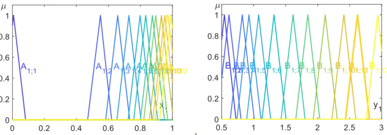
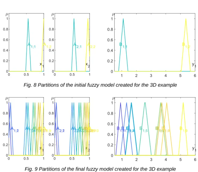
The data sample consisted of 441 input-output pairs, which were randomly divided into two groups (see Fig. 7). The first group containing 80% (353 tuples) of the original sample was used for training of the fuzzy system, while the second group containing the rest of the data points was reserved for test purposes. The VLESFRI [5] fuzzy inference technique was used for the model. The performance of the initial model with two rules was PIRMSEP=14.78%. Its partitions are presented in Fig. 8. At the end of the tuning process the final fuzzy model consisted of 17 rules and its performance in case of the training data was PIRMSEP=4.61% while in case of the test data set it provided PIRMSEP=4.93%, which can be considered as good result. The partitions of the final model can be seen in Fig. 9.
Fig. 7 Two-variable test function (left) and sample data points (right)
Fig. 8 Partitions of the initial fuzzy model created for the 3D example
Fig. 9 Partitions of the final fuzzy model created for the 3D example
Fig. 10 shows the variation of the system performance against the training data in course of the tuning process.
Fig. 10 Variation of the performance (RMSEP) in course of the tuning process of the first (2D) fuzzy model
5 Conclusions
The experimental results showed that the presented method was able to produce a low
the presented approach in case of fuzzy controllers [13][3], path planning [15], and human-robot interaction [11].
Acknowledgment
This research is supported by EFOP-3.6.1-16-2016-00006 "The development and enhancement of the research potential at John von Neumann University" project. The Project is supported by the Hungarian Government and co-financed by the European Social Fund.
References
[1] P. Baranyi, L.T. Kóczy, and T.D. Gedeon, “A Generalized Concept for Fuzzy Rule Interpolation,” in IEEE Transaction on Fuzzy Systems, ISSN 1063-6706, Vol. 12, No. 6, 2004, pp 820-837.
https://doi.org/10.1109/TFUZZ.2004.836085
[2] B. Bouchon-Meunier, C. Marsala, and M. Rifqi, “Interpolative reasoning based on graduality,” in Proceedings of the FUZZ-IEEE'2000, San Antonio, USA, 2000, pp. 483-487. https://doi.org/10.1109/FUZZY.2000.838707 [3] E.H. Guechi, J. Lauber, M. Dambrine, G. Klančar and S. Blažič (2010): PDC control design for non-holonomic
wheeled mobile robots with delayed outputs, Journal of Intelligent and Robotic Systems, vol. 60, no. 3-4, pp. 395- 414, Dec. 2010. https://doi.org/10.1007/s10846-010-9420-0
[4] Z.H. Huang, and Q. Shen, “Fuzzy interpolation with generalized representative values,” in Proceedings of the UK Workshop on Computational Intelligence, 2004, pp. 161-171. http://hdl.handle.net/2160/429
[5] Z.C. Johanyák: Performance Improvement of the Fuzzy Rule Interpolation Method LESFRI In: Szakál, Anikó (Ed.) CINTI 2011 - 12th IEEE International Symposium on Computational Intelligence and Informatics, IEEE, (2011), pp. 271-276., https://doi.org/10.1109/CINTI.2011.6108512
[6] Z.C. Johanyák, A. Kőházi-Kis: Incremental Fuzzy Rule Base Extension with Optimization, A GAMF Közleményei, Kecskemét, XXIV. (2010-2011), HU ISSN 1587-4400, pp. 23-34.
[7] Johanyák, Z. C., Kovács, S.: Sparse Fuzzy System Generation by Rule Base Extension, 11th IEEE International Conference of Intelligent Engineering Systems (IEEE INES 2007), June 29 - July 1, 2007, Budapest, pp. 99-104, https://doi.org/10.1109/INES.2007.4283680
[8] Kennedy, J., Eberhart, R., 1995, Particle Swarm Optimization. in Proceedings of IEEE International Conference on Neural Networks IV., Perth, 1995, 1942–1948., https://doi.org/10.1109/ICNN.1995.488968
[9] L. Kovács, “Rule approximation in metric spaces,” Proceedings of 8th IEEE International Symposium on Applied Machine Intelligence and Informatics SAMI 2010, Herl'any, Slovakia, pp. 49-52.,
https://doi.org/10.1109/SAMI.2010.5423702
[10] S. Kovács, “Extending the Fuzzy Rule Interpolation "FIVE" by Fuzzy Observation,” Advances in Soft Computing, Computational Intelligence, Theory and Applications, Bernd Reusch (Ed.), Springer Germany, 2006, pp. 485-497., https://doi.org/10.1007/3-540-34783-6_48
[11] S. Kovács, D. Vincze, M. Gácsi, Á. Miklósi and P. Korondi, "Fuzzy automaton based Human-Robot Interaction,"
2010 IEEE 8th International Symposium on Applied Machine Intelligence and Informatics (SAMI), 2010, pp. 165- 169, https://doi.org/10.1109/SAMI.2010.5423746.
[12] R.-E. Precup and R.-C. David, Nature-Inspired Optimization Algorithms for Fuzzy Controlled Servo Systems.
Oxford, UK: Butterworth-Heinemann, Elsevier, 2019. https://doi.org/10.1016/C2018-0-00098-5
[13] R.-E. Precup and S. Preitl, Development of fuzzy controllers with non-homogeneous dynamics for integral-type plants, Electrical Engineering, vol. 85, no. 3, pp. 155-168, Jul. 2003. https://doi.org/10.1007/S00202-003-0157-7 [14] D. Tikk, I Joó, L T Kóczy, P Várlaki, B Moser and T D Gedeon: Stability of interpolative fuzzy KH controllers,INT J
FUZZ SET 125:5-119 (2002). https://doi.org/10.1016/S0165-0114(00)00104-4
[15] J. Vaščák and M. Rutrich, Path planning in dynamic environment using fuzzy cognitive maps, Proceedings of 6th International Symposium on Applied Machine Intelligence and Informatics (SAMI 2008), Herľany, Slovakia, 2008, pp. 5-9. https://doi.org/10.1109/SAMI.2008.4469153
[16] K.W. Wong, D. Tikk, T.D. Gedeon and L.T. Kóczy, “Fuzzy rule interpolation for multidimensional input spaces with applications”. IEEE Trans on Fuzzy Sys. , 13(6), 2005, pp. 809–819., https://doi.org/10.1109/TFUZZ.2005.859316