Improved mixing rates of directed cycles by added connection
Bal´ azs Gerencs´ er
∗Julien M. Hendrickx
†October 8, 2018
Abstract
We investigate the mixing rate of a Markov chain where a combination of long distance edges and non-reversibility is introduced: as a first step, we focus here on the following graphs: starting from the cycle graph, we select random nodes and add all edges connecting them. We prove a square factor improvement of the mixing rate compared to the reversible version of the Markov chain.
Keywords: mixing rate, random graph, non-reversibility.
1 Introduction
We study the mixing properties of certain Markov chains which describe how fast the distribution of the state approaches the stationary distribution regardless of the initial conditions. The overall goal is to provide significant improvement of mixing by minor modifications of the Markov chain.
Mixing time and rate are fundamental quantities in the study of Markov chains [9], [12] and are the object of active research; they are also highly relevant to applications where mixing properties are strongly tied with performance metrics. This is for example the case for Markov chain Monte Carlo methods, which provide cheap approximations for integrals, and also allow sampling from complex distributions that would otherwise be hard to generate directly [7]. Markov chains also provide a powerful scheme for approximating the volumes of high dimensional convex bodies [10], [11]. A different application, average consensus, involves the distributed computation of the average of initial values at different agents in a multi-agent system (values which might correspond to measurements, opinions, etc.) [16]. This can be achieved using a Markov chain for which the stationary distribution is uniform. The initial values can be viewed as a probability distribution scaled by a constant, and the Markov chain will approach the uniform distribution multiplied by the same constant, therefore the average of the initial values will be present at each node. Efficient consensus (and average consensus) approaches actually also play a role in several recent distributed optimization algorithms [13], [14]. For all these applications good performance is crucial and it is determined by the dynamics of the underlying Markov chain. Mixing properties are formulated exactly to answer such questions, which are the topic of the current paper.
There are several ways of obtaining good mixing performance. In many applications, the graph of possible transitions is determined by the problem definition, but the specific transition probabilities can be chosen. When these are required to satisfy some strong symmetry properties (reversibility, described later in detail) choosing those to optimize the mixing rate can be formulated as an SDP problem [2], [3], which can be solved numerically using standard methods. Departing from these symmetry properties brings strong technical challenges, at the same time it can actually lead to significant improvement; the mixing time can indeed drop to its square root in some cases [4], [12]. On the other hand, when it is possible to modify the
∗B. Gerencs´er is with MTA Alfr´ed R´enyi Institute of Mathematics, Hungary,gerencser.balazs@renyi.mta.huHe is supported by NKFIH (National Research, Development and Innovation Office) grant PD 121107. This work has been carried out during his stay at Universit´e catholique de Louvain, Belgium.
†J. M. Hendrickx is with ICTEAM Institute, Universit´e catholique de Louvain, Belgium, julien.hendrickx@uclouvain.be The work is supported by the DYSCO Network (Dynamical Systems, Control, and Optimization), funded by the Interuniversity Attraction Poles Programme, initiated by the Belgian Federal Science Policy Office, and by the Concerted Research Action (ARC) of the French Community of Belgium.
arXiv:1509.01431v4 [math.PR] 10 Feb 2018
graph of possible transitions, astonishing speedup can also be obtained by adding even a small number of randomly selected edges [1], [5], [8].
Our long term goal is to study the speedup that can be achieved by a combination of two a priori orthogonal transformations: (i) the addition of a small number of random edges, and (ii) the introduction of a strong non-reversibility. We start with a cycle graph ofn nodes, select a lower number k of them to become hubs, then add extra edges between the hubs. This scheme is motivated by one of the renown models to represent Small World Networks, the Newman-Watts model [5], [15]. The cycle presents a natural way of including asymmetry by introducing adrift meaning increased clockwise transition probabilities along the cycle and decreased counter-clockwise ones. At this stage the model needs three parameters to be specified:
the placement of the hubs, the added interconnection structure on them, and the asymmetry introduced along the cycle.
In this paper we consider as a first step a model where hubs are chosen randomly,all edges between hubs are included and asymmetry is taken to the extreme: the Markov chain is a pure drift along the cycle taking deterministic clockwise steps, except at the hubs. To better understand the dynamics of the process, observe that the state of the Markov chain can be described by an arc (as the cycle is split by the hubs) and the position within that arc. The main challenge here is to show mixing happens both in term of arcs and in terms of positions within. We prove that this model reaches a mixing rate of Ω(k/n) (up to lognfactors) if k=nσ.
In comparison, if we were to put pure drift along the cycle but with equidistant hubs, we would have rapid mixing in term of the arcs (a perfect one after leaving the first arc), but no mixing at all in term of the position on the arc. Even by decreasing the drift or changing the interconnection structure, the mixing rate will remainO((k/n)2) [6].
Furthermore, if we were to stay with the classical, symmetrical transitions along the cycle, the mixing rate will be againO((k/n)2): for an arc at least n/k long even the hitting time of the ends of the arc from the middle is Ω((n/k)2). This holds for any hub placement and interconnection structure.
After all, we want to emphasize that a speedup with a mixing rate of Ω(k/n) is feasible only now that both random hubs and a drift along the cycle are implemented, as opposed to only one of these.
The rest of the paper is organized as follows. In Section 2 we formally describe the random graph model and Markov chain on which we focus and a proxy graph model that we will use for the analysis. In Section 3 we prove the main mixing rate result for this proxy graph model. We then translate our result to the primary graph model in Section 4. In Section 5 simulations are presented complementing our asymptotic analytical results. We also demonstrate how the mixing rate changes when the drift is decreased for the model, suggesting that further performance improvements might be possible. We draw conclusions and outline possible future research directions in Section 6.
2 Graph models, Markov chains and mixing rates
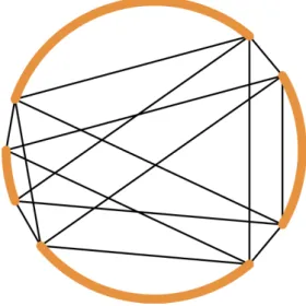
The concept of the graphs we consider is the following. We start with a cycle withnnodes, and randomly select a low number of vertices,nσ out of the total ofnfor some 0< σ <1, which become hubs. Then we connect all hub nodes with each other. Let us now present the precise definitions.
Definition 1. Given n, k∈Z+ we define the random graph distributionBn(k) as follows. Starting from a cycle graph onnnodes, we randomly uniformly choose among thekelement subsets of edges and we remove the edges in the chosen subset. For theith remaining arcs, 1≤i≤k, we mark the clockwise endpoint asai
and the other end asbi. Then we add all edges (bi, aj), for all 1≤i, j≤k. An example is given in Figure 1.
We are interested in the mixing behavior of Markov chains on these graphs. A Markov chain isreversible if for any edge (u, v) of the graph the probability of theu→vtransition is the same as thev→utransition.
In this paper we go further from the comfortable domain of reversible Markov chains, let us now introduce the ones we will focus on.
Definition 2. For any graph coming fromBn(k) we define thepure drift Markov chain as follows. Within any arc we set transition probabilities to 1 along the arc all the way from ai to bi. From any bi, we set transition probabilities to 1/kon all edges towards allaj. A part of such a chain is visualized in Figure 2.
Figure 1: Example graph fromBn(k) (see Definition 1).
Figure 2: Example arc from the pure drift Markov chain (see Definition 2).
This is a Markov chain which has a doubly stochastic transition matrix, therefore the stationary distri- bution is uniform. We want to analyze the asymptotic rate as the distribution approaches the stationary distribution. This mixing performance of the Markov chain will be measured by the mixing rate:
Definition 3. For a Markov chain with transition matrixP we define themixing rate λas λ= min{1− |µ| : µ6= 1 is an eigenvalue ofP}.
Observe that for large numbers of nodes and comparably low number of hubs, arc lengths approximately follow a geometric distribution. However, they are not independently distributed, and this approximation is not valid for large lengths. Hence we introduce an alternative, simpler model of graphs reflecting ap- proximately the same concept but technically more convenient due to the added independence. We will first establish our result for this alternative model, and then extend it in Section 4 to the original model of Definition 1.
Definition 4. Given L ∈(1,∞), k ∈ Z+, we define the random graph distribution B(L, k). Let us take independentlykrandom variables
Li∼Geo(1/L), i= 1, . . . , k,
where Geo(p) denotes a geometric random distribution with parameter p (and 1 as the smallest possible value). We begin with a graph that is the disjoint union ofkarcs, paths withLi nodes, each of which has a
“start point”aiand an “end point”bi, withai=biifLi= 1. Then we add all edges (bi, aj), for 1≤i, j≤k.
The extension of the pure drift Markov chain (Definition 2) to this graph model is immediate. Note that we chose to haveLi denote the number of nodes as opposed to the length of the path, because it leads to simpler expressions in the technical developments.
3 Random polynomials for pure drift Markov chains
In order to find the mixing rate of a Markov chain, we have to know the eigenvalues of its transition matrix.
For the current case we transform this eigenvalue problem into finding the roots of a certain polynomial.
Proposition 5. Let us consider the pure drift Markov chain on a random graph fromB(L, k). Define also
q(z) =
k
X
i=1
z−Li. (1)
Then for µ6= 0,µ∈C is an eigenvalue of the transition matrixP if and only ifq(µ) =k.
Proof. Assuming µ is the eigenvalue of the transition matrix P let us find the corresponding eigenvector x. Observe that each ai has incoming edges from exactly the same nodes and the same weights, so the eigenvector must take the same valuexai =hat each of them for someh.
For two subsequent nodespandp+ along an arc, fromxP =µxwe get xp=µxp+.
This implies that along the arcs we see the valuesh, hµ−1, . . . , hµ−Li+1 (and thus justhin case of a single node arc). This already completely determines xup to scaling and ensures the eigenvalue equation for all nodes except theai. We get a valid eigenvector if the equation also holds forai, which takes the form
k
X
i=1
1
khµ−Li+1=µh.
Having a non-zero eigenvector implies h 6= 0. Therefore the above equation is equivalent to q(µ) = k if µ6= 0.
For the other direction, given aµ6= 0 such thatq(µ) =k, we can again buildxby setting 1, µ−1, . . . , µ−Li+1 on each arc, and this will clearly be an eigenvector ofP with eigenvalue µ.
By Definition 3, the mixing rate is high if the transition matrix P has no eigenvalue near the complex unit circle. Therefore to get a lower bound on the mixing rate we have to exclude a ring shaped domain for the eigenvalues. The region to be avoided is
Rγ =
z: 1− 1
Llogγk ≤ |z| ≤1, z6= 1
, (2)
whereγis a constant parameter to be chosen later. We will show that asymptotically almost surely (a.a.s.) no eigenvalue ofP falls inRγ. The width of the ring should be viewed as follows. We assumeLandkare of similar magnitudes meaning that they have a polynomial growth rate w.r.t. each other. Therefore the width is at most a logarithmic factor lower than 1/L. Our key result is the following:
Theorem 6. Assume k, L→ ∞ whileρl<logL/logk < ρu for some constants0< ρl< ρu <∞, and fix γ >4. We use the graph model B(L, k) and the definition ofq(z)from (1) andRγ from (2). Then for any c, d >0 we have
P(∃z∈Rγ, q(z) =k) =O(k−cL−d).
Consequently, in view of Proposition 5 and the definition ofRγ, we obtain for the mixing rateλ >1/(Llogγk) a.a.s.
We show the claim in four steps. First we ensure that we can assume the Li variables to be bounded with high probability, this will make further estimates possible. We then checkzcoming from different parts ofRγ: we start with positive reals, then we treat complex numbers in two different ways depending on their arguments.
Intuitively the reason is the following. For some real 0< z <1,q(z) will be too large. Next, takez with low arguments, now all z−Li will be in the same half-plane resulting in a non-zero imaginary part for q(z).
When the argument is far enough such thatq(z) has a chance to have zero imaginary part again, thez−Li will point in various different directions so that the cancellations will force the real part belowk, a.a.s.
Now let us make all this precise. We will confirm that each of the intuitive steps above work with high probability, with the fourth requiring theLito be different enough and not being extremely large. We then join these steps to give a proof of the theorem.
The probabilistic upper bound we need on theLi can be formulated in the following way:
Lemma 7. For anyC >1, L≥2, there holds P(max
i Li≥CLlogk) =O k1−C .
Proof. Assumek≥2. Remember thatLi are i.i.d. variables with lawGeo(1/L). Therefore we have that P(Li≥CLlogk) =P(Li≥ dCLlogke) =
1− 1
L
dCLlogke−1
≤2
1− 1 L
CLlogk
,
based on 1−L1dCLlogke
≤ 1−L1CLlogk
and 1−L1−1
<2. Knowing (1−1/L)L<1/e we get P(Li ≥CLlogk)≤2e−Clogk = 2k−C.
To treat allLi together for 1≤i≤k, we us a simple union bound.
P(max
i Li≥CLlogk)≤2k1−C.
From now on, we will only investigate the (a.a.s.) event that the maximalLi is small as shown in Lemma 7. Let us call this event S(C). We now checkz coming from different parts of Rγ. The simplest case is whenz is a positive real:
Lemma 8. Assume z∈(0,1). Thenq(z)6=k.
Proof. For suchz,q(z) is composed ofk positive termsz−Li, each of them being larger than 1 because all Li are positive (Remember that the smallest possible value for the numbers of nodesLiis 1). Consequently the sum of thez−Li is higher thank.
Next we show that there is noz∈Rγ with small arguments for whichq(z) =k.
Lemma 9. Assume S(C) and take z ∈ Rγ such that 0 6= |arg(z)| < π/(CLlogk). Then =q(z) 6= 0.
Consequently q(z)6=k.
Proof. Without loss of generality, assume arg(z)>0. The event S(C) ensures 0 < Li < CLlogk, so the z−Li will all be in the same half-plane, as they will have an argument in (−π,0). For all these values, the imaginary part is negative, and the same holds thus true for their sum. Therefore it simply cannot be 0.
It remains to check the elements ofRγ whose argument is “large”. The arguments in question are those in
A:=
π
CLlogk,2π− π CLlogk
. (3)
We argue that the arguments of z−Li become so different that strong cancellations will happen. We now formalize this idea in terms of the sum of cosines of the argumentsLix. Note that the proposition statement uses cos+(y) = max(cos(y),0) instead of simple cosines because we will need to take the sums of cos+scaled by different magnitudes
z−Li
in (14).
Proposition 10. Choose constantsα, β >1and alsoρl, ρu as in Theorem 6, and requireρl<logL/logk <
ρu, wherek, L, Li, defined in Definition 4, are the number of arcs, the expected arc length, and the actual lengths of the arcs. We define
m=dlogαke, δ= log−βk.
Then for k, Llarge enough we have,
P sup
x∈A m
X
i=1
cos+(Lix)< m−δ2
!
≥1 3, wherecos+(y) = max(cos(y),0).
Proof. Broadly speaking we will show that at least one of theLixterms will be far from 2kπ, which should decrease enough the sum of the cosines. For a singlex, we state the following lemma.
Lemma 11. Usek, L, Li as in Definition 4. Fix β >1,x∈A (as defined in (3)) and choose an arbitrary modulo 2πinterval D⊂[0,2π]of size |D|= 6δ= 6 log−βk. Then fork, L large enough we have
P({L1x} ∈D)≤2 3, where{a}stands fora mod 2π.
Proof. Each element of the series{x},{2x},{3x}, . . .is either inDor not. We can therefore split the series into blocks that are inDand to blocks that are not. Lett1 be the first coefficient such that{t1x} ∈D, then we can define the blocks
{tix},{(ti+ 1)x}, . . . ,{(si−1)x} ∈D, {six},{(si+ 1)x}, . . . ,{(ti+1−1)x}∈/ D, withsi≥ti+ 1 andti+1≥si+ 1. Observe that
P({L1x} ∈D) =X
i≥1
P(L1∈[ti, si−1]) (4)
= 1−X
i≥1
P(L1∈[si, ti+1−1])−P(L1< t1)
≤1−X
i≥1
P(L1∈[si, ti+1−1]).
We will now show
P(L1∈[ti, si−1])≤2P(L1∈[si, ti+1−1]), (5) which together with (4) will allow to conclude.
For this purpose, we first compare the number of elements in the blocks above by relatingti+1−si with si−ti. We claim fork, Llarge enough that
ti+i−si ≥si−ti. (6)
Indeed, for suchk we have|D|= 6δ < π/2. Without the loss of generality we assumex∈[0, π].
Ifsi−ti= 1, then we immediately getti+i−si≥si−ti. Otherwise, there are at least two consecutive elements of the series inD and the length 6δofD is thus at least (si−ti−1)x. Therefore we have
x≤ 6δ
si−ti−1 ≤ π
2(si−ti−1). (7)
A simple consequence isx≤6δ≤π/2. Also, by rearranging we get x(si−ti)≤π
2 +x. (8)
For the elements outsideD, observe that since (si−1)xis inDandti+1xis again inD, theti+1−siintervals of lengthxdefined by [(si−1)x, six],[six,(si+ 1)x], . . . ,[(ti+1−1)x, ti+1x] must cover at least the length of the complement ofD, i.e. at least 2π−6δ. We have thus
ti+1−si≥ 2π−6δ x −1≥
3 2π
x −1.
Rearranging yields
x(ti+1−si)≥ 3π 2 −x.
We compare this with (8), note that 0< x≤π/2 and conclude again thatti+i−si≥si−ti.
We now show an upper bound on the block sizes. Remember thatx∈Adefined in (3) impliesx≥ CLπlogk. So using (7) andδ= logβk, we obtain
si−ti ≤6δ
x + 1≤ 6δ
π/CLlogk+ 1 = 6
logβk· CLlogk
π + 1≤2CLlog1−βk+ 1. (9) Let us come back to the probabilities ofL1falling within the blocks defined. AsL1is a geometric random variable, shifting the interval of interest bysi−ti introduces only a simple multiplicative factor:
P(L1∈[ti, si−1]) =
1− 1 L
ti−si
P(L1∈[si, si+ (si−ti)−1])≤. . .
We enlarge the target interval from lengthsi−ti toti+1−si relying on (6). Clearly by this the probability cannot decrease.
. . .≤
1− 1 L
ti−si
P(L1∈[si, ti+1−1]). (10) For the coefficient at the end of (10) we use (9) to get for k, Llarge enough
1− 1
L ti−si
≤
1− 1 L
−2CLlog1−βk−1
≤exp(3Clog1−βk)
1 + 2 L
≤2.
During these estimates we used (1−1/L)−2L ≤exp(3) and (1− L1)−1 ≤ 1 + L2 for L large enough, and log1−βkbeing as close to 0 as needed for klarge enough.
Substituting this last bound together into (10) leads to (5). This is enough to complete the proof as we have seen before.
To come back to the proof of Proposition 10, let us chooseD= [−3δ,3δ]. For small enoughδ, whenever we have {Lix} ∈/ D, it implies cos+(Lix) <1−2δ2. Assuming δ to be small enough is again equivalent to another (independent) bound fork to be large enough. Using Lemma 11 and knowing that the Li are independent random variables we have
P
m
X
i=1
cos+(Lix)≥m−2δ2
!
≤P({Lix} ∈D)m≤ 2
3 m
, (11)
where m = logαk was defined in the statement of the proposition. This is the type of probability bound we are looking for, but only for a single x. Next we extend it to all x∈A simultaneously, whereA is the interval of interest of arguments (3). As an intermediate step, breakA into dA/e equal subintervals with = 2δ2/(mCLlogk) and choosexj as the middle of each of these subintervals. In this setting, no point of Ais further than/2 from some pointxj. Using the union bound for these chosen points we see
P sup
j m
X
i=1
cos+(Lixj)≥m−2δ2
!
≤X
j
P
m
X
i=1
cos+(Lixj)≥m−2δ2
!
Taking into account the number of pointsxj in the grid and (11), we obtain P sup
j m
X
i=1
cos+(Lixj)≥m−2δ2
!
≤
2πmCLlogk 2δ2
2 3
m
≤π(logαk+ 1)CLlogklog2βk 2
3 logαk
=CπLlog2β+α+1k 2
3 logαk
(1 +o(1)).
(12)
In this final term (2/3)logαk decreases faster than the inverse of any polynomial ink as α > 1. All others parts of the product have polynomial or lower rate in k. Consequently we see that the right hand side of (12) will become arbitrarily small ask, Lgrows. In particular, it will go below 2/3.
At this point we have the probability estimate for grid pointsxj. We need to extend this to the complete intervalA, introduced in (3). We show that fork, Llarge enough we have
P sup
x∈A m
X
i=1
cos+(Lix)≥m−δ2
!
< P sup
j m
X
i=1
cos+(Lixj)≥m−2δ2
!
. (13)
Indeed, for any x∈ A there is a grid point xj at most /2 away. As the derivative of cos+ stays within [−1,1], the change of the sum when moving toxj fromxis at most
m
X
i=1
2Li≤m δ2
mCLlogkCLlogk=δ2.
Therefore when the sum on the left hand side of (13) is at least m−δ2 for a certain x ∈ A then there also must be a grid point xj for which the sum is at least m−2δ2. The inclusion of the events shows the inequality for the probabilities.
Proof of Theorem 6. Note that the right hand side of the claim can be slightly simplified. The relation betweenL and kensureskρl < L < kρu after a while, therefore the Lterm on the right hand side can be replaced by a power ofk. It is now sufficient to show that the probability in question isO(k−c) for allc >0, we will thus consider only this case.
Choose C ≥ c+ 1. Let us assume maxiLi < CLlogk. This not being true is an exceptional event of probability O(k−c) as shown in Lemma 7. In order to exclude the roots from allRγ, we split this region into three parts, and show thatz cannot be a solution ofq(z) =kin any of these parts.
When 0< z <1 is a positive real, it cannot be a solution according to Lemma 8. Whenz has a small argument, that is,|arg(z)|< π/(CLlogk), we refer to Lemma 9 to confirmz cannot be a solution either.
The remaining case is when z has a large argument, that is, arg(z)∈A. We aim to bound <q(z). On one hand, we estimate the magnitude of the terms z−Li. Then we combine these with the cosines of the arguments to find their contributions to the real part of q(z). Here we rely on Proposition 10, but let us make this precise.
We need to check the magnitude of the termsz−Li. Knowing|z|>1−1/(Llogγk) and Li < CLlogk fork, Llarge enough we have
|z|−Li ≤
1− 1
Llogγk
−CLlogk
≤
1 + 2
Llogγk
CLlogk
≤exp(2Clog1−γk)≤1 + 4C logγ−1k. Considering<q(z), this gives
<q(z) =
k
X
i=1
|z|−Licos(Lix)≤
k
X
i=1
|z|−Licos+(Lix)≤
1 + 4C logγ−1k
k X
i=1
cos+(Lix). (14) Note that the last inequality is the reason we have been working with cos+, as it would generally not hold true for cos. Let us arrange the k elements of this sum into groups of m = logαk arbitrary elements,
consequently resulting ink/m such groups. For a moment we assume k is divisible bym. Let the sum of these groups beS1, S2, . . . , Sk/m. According to Proposition 10 we have
P(Si≥m−δ2)≤2 3,
and each of these events are independent. Therefore the number of such events happening follows a Binom(k/m, r) distribution for somer≤2/3. From standard Chernoff bounds we see that
P
Binom k
m, r
> 3k 4m
≤P
Binom k
m,2 3
> 3k 4m
≤exp
− k 96m
< k−c,
forklarge enough. Consequently, at most 3k/(4m) ofSi are larger thanm−δ2. (with the exception of an event with probability ofO(k−c)). In this case we have
k
X
i=1
cos+(Lix) =
k/m
X
j=1
Sj ≤ 3k
4mm+ k
4m(m−δ2) =k−δ2k 4m. Plugging this back into (14) we arrive at
<q(z)≤
1 + 4C logγ−1k
k
1− δ2
4m
=k
1 + 4C
logγ−1k 1− 1 4 log2β+αk
. (15)
Let us chooseγ >2β+α+ 1. With such a choice, the term kabove gets multiplied by a coefficient lower than 1 fork large enough. This shows<q(z)< k which impliesz is not a solution ofq(z) =k. This a.a.s.
holds simultaneously for allz∈Rγ, arg(z)∈A.
For the sake of completeness, ifkwas not divisible bym, we could still form bmkcgroups as before with
¯k=mbmkcelements, then collect the sum of the remainingk−k¯ terms intoSbk
mc+1. Performing the same argument and using the trivial upper bound for cos+ when working withSbk
mc+1 we get
<q(z)≤k¯
1 + 4C
logγ−1k 1− 1 4 log2β+αk
+ (k−¯k)
1 + 4C logγ−1k
.
Knowingk−¯k < mthe new additive term compared to (15) is (poly)logarithmic, which will not compensate for the almost lineark/logktype of loss originating from the first term. Hence once again, the right hand side will not reachkand thusz can not be a solution.
Regarding the parameters, previously for Proposition 10 we only needed to ensure α, β >1. Therefore we can apply Proposition 10 and this reasoning for α=β = 1 +, γ = 4 + 4 for any > 0, eventually allowing anyγ >4.
Remember that during the proof, we had two small exceptional events, both having probabilityO(k−c).
This allows thus confirming the theorem with the condition on γ and with the probability bound on the exceptional cases.
Theorem 6 guarantees the absence of eigenvalues with large absolute value (except at 1) with high probability. We can reformulate it in the following way
Theorem 12. Assume k, L→ ∞whileρl<logL/logk < ρu for some constants 0< ρl< ρu <∞. Then for any γ >4 a.a.s. we have the following bound on the mixing rate for B(L, k):
λ > 1 Llogγk.
Proof. This lower bound is a direct consequence of Theorem 6 and the definitions ofRγ and the mixing rate λ.
4 Mixing rates for B
n(k)
We now translate Theorem 12 to our initial graph modelBn(k), where the total number of nodes are fixed beforehand. For this purpose, we first show that for any L ∈ R+ the conditional distribution of B(L, k) conditioned on havingnnodes in total is the same asBn(k) in the following sense. We will use the compact notationB(L, k)|n for the aforementioned conditional distribution.
We need to map a graph fromB(L, k)|nto the cycle. Given such a graphG(as we build it in Definition 4) ands∈ {1,2, . . . n}= [n] defineT(G, s) as follows. Mapa1 to nodes, then progressing along the arc of L1 tos+ 1, s+ 2, . . ., continuing withL2, L3, . . .taking the numberss+imodulononce needed. Map the edges ofGconsistently with the nodes, thenT(G, n) is a graph on the labeled nodes [n].
Proposition 13. Given are n, k ∈ Z+, L ∈ R+. Let U(n) denote the uniform distribution on [n] and T∗(·,·) the induced measure transformation ofT(·,·)defined above.
ThenT∗(B(L, k)|n, U(n)) =Bn(k). Simply speaking, if we randomly choose the starting point where we map B(L, k)|n to the cycle, we get the distribution Bn(k).
Note that the randomization in the mapping does not change the internal structure of the graph, therefore once the proposition is proven, we also immediately get the following:
Corollary 14. Given n, k ∈Z+, L∈R+ consider the conditional distribution B(L, k)|n. Then the corre- sponding distribution of the mixing rate λis the same as the distribution ofλforBn(k).
Proof of Proposition 13. For any l1 ≥ 1 we have P(L1 = l1) = (1−p)l1−1p and the arc of a1· · ·b1 will consist of l1 nodes, (withp= L1). Consequently, in the setup of{L1 =l1, L2 =l2, . . . , Lk =lk} we get a total ofnnodes exactly ifPk
i=1li=n. The probability of such an instance is P(L1=l1, L2=l2, . . . , Lk =lk) =
k
Y
i=1
(1−p)li−1p= (1−p)Pki=1lipk = (1−p)n−kpk.
This probability is independent of the choice of{Li}ki=1, therefore the conditional distribution is uniform on all the possibilities.
A uniform number on [n] is supplemented and we need to relate this joint variable to the distribution of Bn(k). It is straightforward to see thatT will map any element in the support ofB(L, k)|n×[n] to an element of the support ofBn(k) as they are built the same way.
Moreover, this will be a homogeneous map in the sense that each element of the support of Bn(k) will be obtained exactlyktimes. To see this, start from any such element, we will get the kdifferent preimages depending on which arc we choose to beL1. (Note that two subsequent deleted edges might lead to an “arc”
without edges, of size 1 in our current notation.)
In the end, both the conditional distributionB(L, k)|n andU(n) were uniform, applying the mapT that is a uniformk-fold cover on a target space will result in a uniform distribution on its range, confirming the claim of the proposition.
Our last ingredient is a lower bound on the probability for a random graph model B(n/k, k) to have exactlynnodes.
Lemma 15. The probability for a random graph B(n/k, k)to have exactly nnodes is at least n1.
Proof. We have seen in the proof of Proposition 13 that all instances ofnnodes have the same probability 1−nkn−k k
n
k
. Moreover, standard combinatorial arguments show that there are n−1k−1
ways of distribut- ing thennodes into thekarcs, leading to the following probability of obtaining exactlynnodes, and event that we denote byM(n, k)
P(M(n, k)) = n−1
k−1 k n
k 1−k
n n−k
= n−1
k−1
kk(n−k)n−k
nn . (16)
We develop a simple asymptotic estimate for this probability. From the Stirling formula we know that
n→∞lim
√ n!
2πn nen = 1.
For conciseness, we will use the≈relation if the ratio of the two quantities is 1 in the limit. In this spirit we get
n k
≈
√2πn nen
√2πk kekp
2π(n−k) n−ke n−k =
r n 2πk(n−k)
nn kk(n−k)n−k. Let us plug this back to (16), while noting n−1k−1
= kn nk .
P(M(n, k))≈ k n
r n 2πk(n−k) =
s k 2πn(n−k). As a very crude bound we get forn, k large enough that
P(M(n, k))> 1
n. (17)
We can now extend Theorem 12 to our initial model Bn(k).
Theorem 16. Assume n, k → ∞while ρl <logn/logk < ρu for some constants 1< ρl < ρu<∞. Then for any γ >4 a.a.s. we have the following bound on the mixing rate for Bn(k):
λ > k nlogγk.
Proof. We know from Theorem 6 that the probability of the polynomialq(z) having a root in the forbidden ring (and thus of the mixing rate being smaller than Llog1γk) bounded as O(L−2k−2) = O(n−2). Hence it remains negligible with respect to the probability ofB(n/k, k) having exactlynnodes (forn, klarge enough) which we have shown in Lemma 15 to be at least 1/n. We deduce that the mixing rate of pure drift Markov chains for the conditional random graph model B(n/k, k)|n is also at least Llog1γk a.a.s. Proposition 13 allows then concluding that the same holds forBn(k), which concludes the proof.
5 Simulations
Following the asymptotic theoretical results we perform complementing simulations to analyze the tightness of the bounds obtained. We also explore further using numerical tools for the next step of research that is not yet treated analytically.
The mixing results we have are exciting as we see a strong speedup compared to the similar reversible Markov chain with transition matrix ˜P = (P +P>)/2. By this we set all transition probabilities on all edges to be equal in the two directions. For this Markov chain, if the initial distribution is concentrated in the middle of the longest arc, the Central Limit Theorem ensures that even after Ω(L2log2k) steps the probability of not leaving the arc is bounded away from 0. Consequently we get a lower bound of the same order for the mixing time and which in turn translates to the mixing rate bound
λ < C
L2log2k, (18)
which is a square factor worse than our new results for the non-reversible Markov chain.
Simulations are in line with the speedup we see when comparing (18) with Theorem 12. Figure 3 is a log-log histogram showing the decrease of λ as the node countn increases. The histogram presents the
4 5 6 7 8 -10
-8 -6 -4 -2 0
logn
logλ
Figure 3: Histograms for the mixing rates λ for the Markov chains on the graphs Bn(b√
nc). The upper stripe corresponds to non-reversible Markov chains while the lower one to the reversible variants.
simulation results for the non-reversible and reversible Markov chain and we do observe the strong separation predicted by the theoretical results. The stripe on the top presentsλfor the non-reversible Markov chains while the bottom one corresponds to the reversible ones. Figure 3 is based on 200.000 random Markov chains withnranging from 54 to 2980 and withk=b√
nc. As we are interested in typical behavior of these randomized Markov chains, we discarded the top and bottom 5% of the results for everynconsidered.
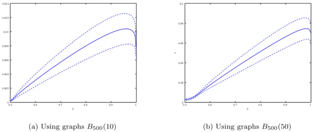
The two type of Markov chains we compared can be seen as the extremal setups: either the asymmetry is so strong that steps are deterministic along the cycle, or we have perfect symmetry. There is however a full spectrum of intermediate situations, and one may wonder which level of asymmetry is optimal. We have seen that full asymmetry is better in terms of mixing performance than full symmetry. On Figure 4, starting from the reversible Markov chain, we gradually change the transition probabilities along the cycle until we reach the current extreme asymmetric case. Specifically, for 1/2 ≤ q ≤ 1 we set the transition matrix Pq =qP + (1−q)P> and compute the mixing rate of the resulting Markov chain. Here we have P1/2 = ˜P , P1 = P as expected. We perform simulations for B500(10) and B500(50). In both case, 8000 random graphs were generated and the mixing rates were computed for all graphs and forq moving along [1/2,1]. Again, the top and bottom 5% were discarded. The means of the resulting mixing rates are presented in Figure 4 together with the sample standard deviations. The figures show that the optimal choice is near the extremal non-reversible case, confirming our concept. Still, interestingly a minor offset towards the reversible version still increases the mixing rate. Intuitively the two effects of the modification match well:
the small loss in the speed of moving along the cycle is well compensated by the local mixing introduced.
The analytic treatment of the intermediate Markov chains for q 6= 1/2,1 brings new challenges as the non-reversible feature is still present while we lose the deterministic nature of the movement along the cycle.
6 Conclusions
We have seen in Theorem 12 and Theorem 16 that for both modelsBn(k) andB(L, k) the mixing rate of the non-reversible Markov chain considered is much higher than the similar reversible one. The results confirm that the simultaneous application of adding long distance edges and also setting the Markov chain to be non-reversible dramatically improves the mixing rate. We believe this phenomenon is promising and could provide similar speedup effects for other reference graphs, other methods to add random edges and other means of introducing non-reversibility.
0.5 0.6 0.7 0.8 0.9 1 0
0.002 0.004 0.006 0.008 0.01 0.012 0.014
p
λ
(a) Using graphsB500(10)
0.5 0.6 0.7 0.8 0.9 1
0 0.02 0.04 0.06 0.08 0.1
p
λ
(b) Using graphsB500(50)
Figure 4: Mixing rates of the transition matricesPq =qP+ (1−q)P>for the interpolation between the pure drift (q = 1) Markov chain and its reversible version (q= 0.5). Solid lines follow the means while dashed lines indicate the sample standard deviations around the means.
We have also seen numerically in Figure 4 that being fully non-reversible is not necessarily optimal in this context, even though it is significantly better than being fully reversible.
Therefore one of the open questions is to find the optimal Markov chain among the intermediate cases.
Another goal for future research is to consider the more realistic situation where the hubs do not have such high number of connection, for instance, by replacing the complete graph on the selectedcnσ nodes with a random matching on them. Simulations similar to Figure 3 in [6] suggest that a similar speedup is to be expected.
References
[1] L. Addario-Berry and T. Lei,The mixing time of the Newman–Watts small world, in Proceedings of the Twenty-Third Annual ACM-SIAM Symposium on Discrete Algorithms, SIAM, 18 Jan 2012, pp. 1661–1668.
[2] S. Boyd, P. Diaconis, P. Parrilo, and L. Xiao, Fastest mixing Markov chain on graphs with symmetries, SIAM J. Optim., 20 (2009), pp. 792–819.
[3] S. Boyd, P. Diaconis, and L. Xiao,Fastest mixing Markov chain on a graph, SIAM Rev., 46 (2004), pp. 667–689 (electronic).
[4] P. Diaconis, S. Holmes, and R. M. Neal,Analysis of a nonreversible Markov chain sampler, Ann.
Appl. Probab., 10 (2000), pp. 726–752.
[5] R. Durrett,Random Graph Dynamics, Cambridge University Press, 2006.
[6] B. Gerencs´er, Mixing times of Markov chains on a cycle with additional long range connections.
arXiv:1401.1692, 2014.
[7] M. Jerrum, Mathematical foundations of the Markov chain Monte Carlo method, in Probabilistic methods for algorithmic discrete mathematics, vol. 16 of Algorithms and Combinatorics, Springer, 1998, pp. 116–165.
[8] M. Krivelevich, D. Reichman, and W. Samotij,Smoothed analysis on connected graphs, SIAM J. Discrete Math., 29 (2015), pp. 1654–1669.
[9] D. Levin, Y. Peres, and E. Wilmer, Markov chains and mixing times, American Mathematical Society, 2009.
[10] L. Lov´asz and S. Vempala, Hit-and-run from a corner, SIAM Journal on Computing, 35 (2006), pp. 985–1005.
[11] ,Simulated annealing in convex bodies and anO∗(n4)volume algorithm, Journal of Computer and System Sciences, 72 (2006), pp. 392–417.
[12] R. Montenegro and P. Tetali,Mathematical aspects of mixing times in Markov chains, Foundations and TrendsR in Theoretical Computer Science, 1 (2006), pp. 237–354.
[13] A. Nedi´c and A. Olshevsky,Distributed optimization over time-varying directed graphs, IEEE Trans- actions on Automatic Control, 60 (2015), pp. 601–615.
[14] A. Nedi´c, A. Ozdaglar, and P. A. Parrilo,Constrained consensus and optimization in multi-agent networks, IEEE Transactions on Automatic Control, 55 (2010), pp. 922–938.
[15] M. Newman, C. Moore, and D. Watts,Mean-field solution of the small-world network model, Phys.
Rev. Lett., 84 (2000), pp. 3201–3204.
[16] A. Olshevsky and J. N. Tsitsiklis,Convergence speed in distributed consensus and averaging, SIAM J. Control Optim., 48 (2009), pp. 33–55.