Time-dependent electric transport in nodal loop semimetals Zolt´an Okv´atovity,

Zolt´an Okv´atovity,^{1, 2,∗} L´aszl´o Oroszl´any,^{3, 2} and Bal´azs D´ora^{1, 2}

1Department of Theoretical Physics Budapest University of Technology and Economics, 1521 Budapest, Hungary

2MTA-BME Lend¨ulet Topology and Correlation Research Group, Budapest University of Technology and Economics, 1521 Budapest, Hungary

3Department of Physics of Complex Systems, ELTE E¨otv¨os Lor´and University, 1117 Budapest, Hungary (Dated: July 23, 2021)

Close to the Fermi energy, nodal loop semimetals have a torus-shaped, strongly anisotropic Fermi surface which affects their transport properties. Here we investigate the non-equilibrium dynamics of nodal loop semimetals by going beyond linear response and determine the time evolution of the current after switching on a homogeneous electric field. The current grows monotonically with time for electric fields perpendicular to the nodal loop plane however it exhibits non-monotonical behavior for field orientations aligned within the plane. After an initial non-universal growth∼Et, the current first reaches a plateau ∼E. Then, for perpendicular directions, it increases while for in-plane directions it decreases with time to another plateau, still∼E. These features arise from interband processes. For long times or strong electric fields, the current grows as∼E^3/2tor∼E³t² for perpendicular or parallel electric fields, respectively. This non-linear response represents an intraband effect where the large number of excited quasiparticles respond to the electric field. Our analytical results are benchmarked by the numerical evaluation of the current from continuum and tight-binding models of nodal loop semimetals.

I. INTRODUCTION

Recently, the investigation of properties of topologi- cally non-trivial states in solids has become one of the main focuses of condensed matter physics. The the- oretical prediction[1] and experimental realization[2] of topological insulators have inspired the prediction of ex- otic phenomena such as the topological magnetoelectric effect[3] and opened the door for exciting new applica- tions in tools for measuring fundamental constants [4], in thermoelectric devices[5], and in architectural elements of spintronics devices[6]. The bulk topological insula- tors, just as ordinary insulators, are characterized by a gap separating the valence and conduction bands. How- ever, in these materials, the topological properties of bulk states, characterized by theZ2invariant[7], guarantee the presence of robust, spin polarized states on the perimeter of samples.

Topology can still impact the properties of systems in the absence of a band gap. The interplay of topol- ogy and symmetry can also stabilize robust features in these so-called topological semimetals [8–10]. In Dirac and Weyl semimetals[8, 11] band degeneracies near the Fermi-level occur at a discrete set of points in the Bril- louin zone. Recently these systems have been intensively studied both theoretically [12] and experimentally cul- minating in several interesting observations such as the chiral anomaly, anomalous Hall conductivity, and Fermi arc surface states[13–16].

The story of topological semimetals does not end with the Dirac and Weyl points. In certain materials, called nodal line semimetals, band crossings can appear not

∗okvatovity.zoltan@ttk.bme.hu

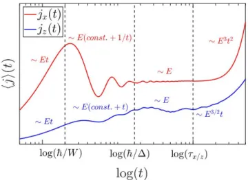
FIG. 1. Schematic picture of the current in nodal loop semimetals when the electric field perpendicular to the nodal loop (blue line) and parallel to it (red line). The black dashed lines represents the timescales which split up the time domain into four different region.

only in selected points but through continuous lines which may form closed loops or traverse the whole Bril- louin zone[8–10]. Stabilizing these nodal lines against gap opening requires the presence of some additional symmetries[10, 17–19].

When the protecting symmetry is broken, either a fi- nite band gap opens or the nodal line breaks into several nodal points in the Brillouin zone. Nodal line semimetals, in general, do not host protected edge states [9], however, localized surface states can appear between the surface projection of the nodal lines [18, 20] called drumhead states. These surface states owing to their dispersion- less nature may provide a fertile ground for correlation-

arXiv:2104.07632v2 [cond-mat.mes-hall] 21 Jul 2021

induced effects[21, 22].

Model systems and material realizations of nodal line semimetals have been recently proposed in hyperhoney- comb structures[23, 24], superlattices made of topological insulators[10, 25], alkaline-earth metal crystals[20, 26, 27]

and cold atomic systems [28, 29].

There has been also intense experimental progress to investigate the surface properties using angle-resolved photoemission spectroscopy (ARPES) [8, 30, 31] or mag- netotransport experiments to reveal the bulk character- istics [32–34]. The characteristic features of nodal line semimetals have been identified in various materials e.g., PbTaSe2 [35, 36], ZrSiTe and ZrSiSe [32, 37] or Ca3P2

[20]. Although the lack of protected edge states makes nodal line semimetals quite challenging to identify ex- perimentally the peculiar nature of their Fermi surface endows them with characteristic electronic and magnetic properties[38–40].

In this paper, we investigate the non-equilibrium dy- namics beyond the linear response of nodal loop semimet- als after a sudden switch of a homogeneous electric field.

We consider a simple continuum model with a single nodal loop located in the (px, py) plane in the momen- tum space at the Fermi level. Following the works in Refs. [41, 42], we provide a detailed derivation of the temporal behavior of the electric current for two dis- tinct cases: when the electric field is perpendicular to the plane of the nodal loop (z direction) or parallel to it (xdirection). The short time/weak electric field limit of the current is obtained using first-order perturbation theory in the electric field while for the long time/strong electric field limit, we use the Dykhne–Davis–Pechukas (DDP) method. The main results are displayed in Fig.

1. We find that in both cases, the time domain splits into four different regions. In the ultrashort regime, the current is linear in time and electric field, and the slope is determined by the high-energy cutoff. In the second region, the current in the z direction reaches a plateau then starts to increase linearly while in the xdirection 1/t decay is observed. For the third region, both cur- rents are constant yet again. This tendency of the current agrees with the suggested behavior from the frequency- dependent optical conductivity from Ref. [43].

In the last temporal regime, the electric field depen- dence of the current becomes non-linear. For the cur- rent, we obtained∼E^3/2tdependence inzdirection and

∼E³t²inxdirection. To test the applicability of our re- sult, we calculated the current by solving the Schr¨odinger equation numerically and also compared it with the cur- rent obtained from tight-binding calculations. The nu- merical results agree well with the time and electric field dependence of the current obtained from analytical calcu- lations. These non-linear features of the electric response are expected to be observable in transport measurements in nodal loop semimetals.

The paper is organized as follows: in Sec. II, we briefly introduce the model Hamiltonian and the current oper- ators. In Secs. III and IV, the temporal and electric

field dependence of the current is investigated when the electric field is perpendicular or parallel with the nodal loop, respectively. Then the results of the tight-binding calculation are detailed in Sec. V. In Sec. VI, the exper- imental possibilities are briefly discussed and in Sec. VII our main results are summarized.

II. MODEL HAMILTONIAN AND OBSERVABLES

We consider the effective low-energy Hamiltonian of a nodal loop semimetal [39] as

H =

"

∆−p²_x+p²_y 2m

#

σ_x+v_Fp_zσ_z=P_xσ_x+P_zσ_z, (1) where σi’s (i = x, z) are the Pauli matrices, m ≈ 0.1−1 me (me is the mass of an electron) is the ef- fective mass [34, 44, 45], ∆ ≈ 0.1 −1 eV is the en- ergy scale that defines the nodal loop radius [46, 47] and v_F≈10⁵−10⁶m/s is the Fermi-velocity in thezdirection [44, 45]. Diagonalizing the Hamiltonian yields the energy spectrum asE_±(p) = ±εp with ± the band index and εp = q

(vFpz)²+ (∆−(p²_x+p²_y)/2m)². The homoge- neous electric field switched on att= 0 is introduced as a time-dependent vector potentialA(t) through the Peierls substitution: p→p−eA(t) att= 0. We are interested in two different cases, when the electric field points tox andzdirection which leads us to two different vector po- tentialsAx(t) = [EtΘ(t),0,0] andAz(t) = [0,0, EtΘ(t)], respectively.

For each momentum pthe Hamiltonian Eq. (1) with the time-dependent vector potential represents a two- level system. Depending on the orientation of the elec- tric field, the instantaneous spectrum exhibits one or two (avoided) level crossings, thus a distinct temporal behav- ior of the electric current in the x and z directions is expected. We investigate the current using the frame- work of the Landau–Zener dynamics [48], with the gen- eral time-dependent Schr¨odinger equation given by

H(t) =Px(t)σx+Pz(t)σz, (2) i~∂tΨp(t) =H(t)Ψp(t). (3) It is convenient to perform a time-dependent unitary transformation first [49], which diagonalizes H(t), and brings us to the adiabatic basis [48]. In the resulting equation, the positive and negative energy eigenstates are readily distinguished, simplifying further analytic and numerical analysis. The unitary transformation is given by

U =

cos ^θ₂^t

sin ^θ₂^t sin ^θ₂^t

−cos ^θ₂^t

, (4)

where tan(θt) =Px(t)/Pz(t). In the adiabatic basis, the Schr¨odinger equation takes the form

i~∂tΦp(t) = [εp(t)σz+F(t)σy] Φp(t), (5)

where Ψp(t) = UΦp(t) and F(t)σy = −i~U⁺∂tU arise due to the explicit time-dependence of the unitary trans- formation. F(t) is referred to as diabatic coupling and is written as [50]

F(t) =~

P_z(t)∂_tP_x(t)−P_x(t)∂_tP_z(t)

2ε²_p(t) . (6)

The initial condition of Eq. (5) corresponds to half filling at zero temperature: Φ^T_p(t = 0) = [0,1]. The current operator for a given momentum in the original basis is defined as jp(t) = ∂H(t)/∂A(t) giving jx(t) = _m^e(px− eEt)σ_x andj_z(t) = −ev_Fσ_z. In the adiabatic basis, the expression for the current operator is

jx(t) = e

m(px−eEt) (sin(θt)σz−cos(θt)σx), (7) j_z(t) =−ev_F(cos(θ_t)σ_z+ sin(θ_t)σ_x). (8) The contribution to the current from a given momentum mode is the expectation value of these operators. By de- noting Φ^T_p(t) = [α(t), β(t)], we introduce the transition probability asnp(t) =|α(t)|² which gives the number of electrons excited from the lower to the upper band (and also number of the holes remaining in the lower band).

The contribution of a given momentum state to the cur- rent expressed with the transition probability reads as

hjxi_p(t) = e

m(px−eEt) sin(θt) (2np(t)−1) + 2εp(t)

E ∂_tn_p(t) (9)

hjzi_p(t) =−evFcos(θt) (2np(t)−1) + 2ε_p(t)

E ∂_tn_p(t) (10)

In both cases, the current consists of an intraband (first term) and interband (second term) part which are also called conduction and polarization current in QED ter- minology, respectively [41, 42, 51]. The total current is given by the momentum integral of the momentum re- solved contributions. We note that thenp(t) independent terms, corresponding to fully occupied or empty states, give no contribution to the current and hence can be omitted. [41, 52]. The properties of n_p(t) and the elec- tric current are discussed in the following sections.

III. CURRENT IN THE Z DIRECTION In this section, the constant electric field is aligned to the z direction i.e., it is perpendicular to the nodal loop. The time-dependent vector potential is A(t) = [0,0, EtΘ(t)], and the variables in Eq. (2) are P_x =

∆−(p²_x+p²_y)/2m which remain time independent and Pz(t) =vF(pz−eEt). The evolution of the instantaneous spectrum is plotted in Fig. 2.

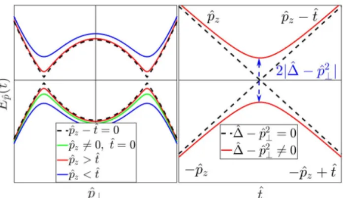
FIG. 2. Visualization of the Landau–Zener dynamics when the E points in the z direction. The gap between the two bands is determined by ˆpzinitially. During the time evolution, the gap starts to decrease and when ˆpz−ˆt= 0 it closes at ˆp⊥=

±p

∆, then start to increase. During the time evolution, theˆ system is driven through a quantum critical point [41].

The time-dependent Schr¨odinger equation and the cur- rent contribution in the adiabatic basis fort >0 read as

i~∂tΦp(t) =

εp(t)σz+~vFeE 2ε²_p(t)

∆− p²_⊥ 2m

σy

Φp(t),

(11) hjzi_p(t) =−evF

vF(pz−eEt)

εp(t) (2np(t)−1) + 2εp(t)

E ∂tnp(t). (12)

Here, we introducedp_⊥ =q

p²_x+p²_y. The scaling prop- erties of the Schr¨odinger equation allow us to introduce dimensionless variables as ˆt = t/τz, ˆ∆ = ∆τz/~,pˆz = vFpzτz/~, ˆp⊥ = p⊥p

τz/2m~ where the scaling factor τz =p

~/evFE defines the natural time scale connected to the electric field. The transition probability behaves differently for ˆt 1 and ˆt 1, which also defines the short- and long-time limits of the total current, respec- tively. As we show below, for short times, the domi- nant contribution to the current is coming from the po- larization part while in the long-time limit, the current is determined by the number of excited electrons in the conduction band [41, 53].

A. Short-time evolution of the current The Schr¨odinger equation in Eq. (11) can be solved an- alytically for arbitrary times and electric fields [51, 54], but it does not give an immediately transparent solu- tion for the transition probability. Therefore it is more practical to obtainnp(t) from approximate solutions in different limits oft. In the short-time limit, employing first-order perturbation theory inE yields the transition

probability as

np(t) = (~vFeE)² 4ε⁶_p

∆− p²_⊥ 2m

² sin²

εpt

~

(13) which is valid except in the close vicinity of the nodal loop i.e. εpvFeEt and resembles closely to the result obtained for graphene [41]. To check the validity of our result, we calculated the transition probability by solving the Schr¨odinger equation in Eq. (11) numerically using the explicit Runge-Kutta method. We obtained good agreement between the analytical and numerical results visualized on the left side of Fig. 3.

FIG. 3. Transition probability for short (left) and long (right) times. The np(t) resembles closely to the transi- tion probability obtained for graphene and Weyl semimetals [41, 42] i.e., dipolar for short times and cylindrical for long times, but shifted to ˆp⊥=±p

∆.ˆ

Using this result in Eq. (12), the conduction part of the current contains already higher (second) order terms in electric field and gives negligible contribution to the total current. Only the polarization current contributes to the linear order in the electric field as

hjzi(t) = v_F²e²E (2π)²~²

Z Λ_z 0

dp_z Z Λ⊥

0

dp_⊥p_⊥(∆−p²_⊥/2m)² ε⁴_p

×sin 2εpt

~

, (14)

Λ_z and Λ_⊥ are the momentum cutoffs which arise from the high-energy cutoffW determined by the bandwidth as W = vFΛz = Λ²_⊥/2m. In Eq. (14), two differ- ent energy scales are present, W and ∆, which in turn

determine three different temporal regions: the ultra- short time transient response, when t ~/W, the sec- ond when~/W t ~/∆ and the third region when

~/∆tp

~/ev_FE.

For the ultrashort time transient response (t~/W), the current is obtained as

hjzi_p(t) = v_F²e²Et (2π)²~³

(∆−p²_⊥/2m)² p(vFpz)²+ (∆−p²_⊥/2m)²³

(15) The momentum integral overp_z andp_⊥ yields

hj_zi(t) = me²v_FE 2π²~³

W tlnh√

2 + 1i

, (16) in the ∆ W limit. This behavior has also been ob- served in Dirac and Weyl fermions [41, 42] with the pic- ture of classical particles accelerated by an external elec- tric field. These particles obey Newton’s equation with the effective mass given bym⁻¹_zz =∂²ε_p(t)/∂p²_z.

In the second region, when~/W t~/∆, the cur- rent saturates to a constant value similarly to graphene [41]. This can be explained by symmetry considerations since for the electric field aligned to the z direction, the cylindrical symmetry of the system remains intact.

Therefore, the nodal loop can be thought of as two ef- fective, graphene-like systems with high-energy cutoffW and ∆, originating from states outside or inside the nodal loop, respectively. Then, the current contribution coming from the first graphene-like system saturates first when

~/W t [41, 42]. With increasing time, an additional linear term in time arises from the second graphene-like system with cutoff ∆. The total current can be approxi- mated as

hjzi(t) = me²vFE (2π)²~²

π² 8 +2t∆

~

. (17)

In the third temporal region, the additional ∆ depen- dent part also saturates, and the current reaches another constant value

hjzi(t) =me²v_FE 16~²

. (18)

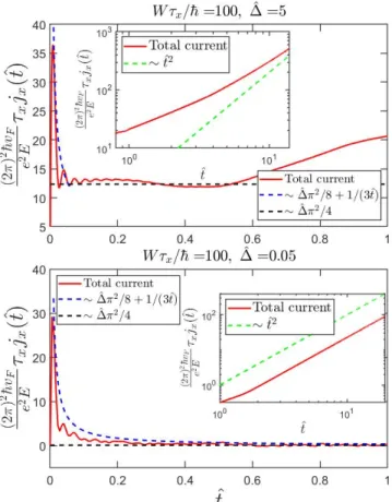
This result allows us to define a dc conductivity by tak- ing the time-independent current in Eq. (18) and di- vide it with the applied electric field as σ_z⁰ = jz/E = me²v_F/16~². This agrees with the optical conductivity at ω →0 in Ref. [43] up to a factor of two, due to the spin degeneracy. As the frequency starts to increase, the optical conductivity decreases with 1/ω while for high frequencies, it tends to a constant valueσ_z⁰/2. All these features in the optical conductivity are in accord with our time-dependent current. Our analytical and numer- ical results agree and are illustrated in Fig. 4.

B. Long-time, strong electric field limit The long time, strong electric field limit, i.e., t p~/evFE is out of the scope of perturbation theory.

FIG. 4. Temporal behavior of the current after switching on the electric field. The blue and black dashed lines rep- resent the polarization current in Eq. (17) and Eq. (18), respectively. When ˆt 1 the conductive current becomes dominant, scaling as∼ˆt.

Although the Schr¨odinger equation can be solved ex- actly for arbitrary times and electric fields in terms of the parabolic cylinder functions [51], it does not pro- vide transparent expressions for the transition probabil- ity and the current. Instead, we rely on the so-called WKB approach to obtain np(t) which is often used to determine transition probability upon tunneling through a barrier [55]. In practice, we use its temporal variant, the Dykhne–Davis–Pechukas (DDP) method [56], which is also known as Landau–Dykhne method for linear time dependence [53].

For longtand largeE, the dispersion relation has lin- ear time dependence with an (avoided) crossing visual- ized in Fig. 2. Then using the DDP method, we obtain for the transition probability [41, 42, 53]

n_p(t) = Θ(p_z)Θ(eEt−p_z) exp

−π(∆−p²_⊥/2m)²

~vFeE

. (19) The exponential term is also called the Schwinger pair production rate [51, 57]. The result in Eq. (19) agrees well with transition probability obtained from numerical calculations, visualized in Fig. 3. Eq. (19) is applicable only when (p_z, p_z−eEt) |∆−p²_⊥/2m|/v_Fholds.

Using this, we calculate the total current, which is dominated by the conductive part as

hjzi(t) =− 2ev²_F (2π)²~³

Z ∞

−∞

dp_z Z ∞

0

dp_⊥p_⊥p_z−eEt εp(t) n_p(t).

(20) We can estimate the overall time and field dependence by rescaling the integral. The transition between bands occurs only if the system is driven through the touching points as plotted in Fig. 2. This holds for 0pzeEt, so the number of excited electrons can be characterized

by a longitudinally growing cylinder of length∼Et[42].

Using the scaling parameterτz, we rescale p_⊥ as ˆp_⊥ = p_⊥p

τz/(2m~) in the second integral of Eq. (20) which brings out an additional ∼ E^1/2 factor. Consequently, the total current should scale with∼E^3/2t.

The integrals over pz andp_⊥ yield

hj_zi(t) =2me²v_FE (2π)²~²

rv_FeE

~ tf_z

√

√ π∆

~v_FeE

(21)

wheref_z(x) = (1 + erf(x))/2 with erf(x), the error func- tion [58]. The time and electric field dependence agree with our estimation from scaling and resembles closely to electric current in graphene [41]. The number of excited particles is given by

N(t) = 1 (2π)³~³

Z

d³p np(t)

= 2meE (2π)²~²

rvFeE

~ tfz

√

√ π∆

~vFeE

, (22)

which leads to hjzi(t) = evFN(t). The current in- creases linearly with time due to the increasing number of electron-hole pairs which propagate with a constantv_F velocity in the conduction and valence band. Due to the nodal loop, an additional ∆ dependent part also arises which is responsible to a factor of 2 enhancement in the electric current. In the ∆ → ∞ or E → 0 limit, due to the structure of the dispersion relation, the electrons can tunnel to twice as many states as in the ∆→ 0 or E→ ∞limit which explains the factor of 2 difference in the electric current, visualized in Fig. 5.

FIG. 5. Schematic plot of the dispersion relation in the

∆ˆ →0 and ˆ∆→ ∞limit. For a given energy (green dashed line) slightly above the gap edge, there are twice as many empty states in the conduction band for ˆ∆ large, therefore the current is 2 times larger.

IV. CURRENT IN THExDIRECTION To calculate the current in the x direction, we use the vector potential A(t) = [EtΘ(t),0,0]. The vari- ables defined in Eq. (2) are Pz = vFpz and Px =

∆eff−(px−eEt)²/2mwhere ∆eff= ∆−p²_y/2m. In con- trast with the previous case, the energy-momentum dis- persion relation has at²temporal dependence fort→ ∞, but the nodal loop is shifted in thexdirection during the time evolution. The temporal behavior of the instanta- neous spectrum is visualized in Fig. 6.

FIG. 6. Left panel: The time evolution of the dispersion relation is illustrated. The time-dependent vector potential shifts the nodal loop in the x direction. Right panel: The time evolution of ˆpxat different values of ˆ∆eff and ˆpz. When

∆ˆeff > 0, ˆpz determines the gap, and ˆ∆eff > 0 sets the lo- cation of the two minimum/maximum points. On the other hand, when ˆ∆eff<0 the gap starts to increase and only one minimum/maximum remains.

The time-dependent Schr¨odinger equation and the electric current contribution for a given momentum mode in the adiabatic basis are given by

i~∂tΦp(t) =

εp(t)σz+~vFeEpz(px−eEt) 2mε²_p(t) σy

Φp(t),

(23) hj_xi_p(t) = e

m

(px−eEt) ε_p(t)

∆_eff−(px−eEt)² 2m

×

×(2np(t)−1) +2εp(t)

E ∂tnp(t). (24) We again introduce dimensionless variables as ˆt =t/τx, where τ_x = p³

2m~/(eE)² coming from the Schr¨odinger equation, giving ˆ∆_eff = ∆_effτ_x/~, ˆp_x/y =p_x/yp

τ_x/2m~ and ˆpz=vFpzτx/~. In order to analyze the Schr¨odinger equation, we apply the same approximations as before, namely first-order perturbation theory for ˆt1 and the DDP method for ˆt1.

A. Short-time and weak electric field limit We again use lowest order perturbation theory to ob- tain the transition probability in the ˆt1 limit.

After some straightforward algebra, we get n_p(t) =

~v_FeE 2m

²p²_xp²_z ε⁶_p sin²

ε_pt

~

(25) which is valid forε_p(eEt)²/2m. The transition prob- ability is evaluated by solving the Schr¨odinger equation in Eq. (23) numerically and is plotted in Fig. 7. For short times and low electric fields, we obtained good agreement between the numerical and analytical result.

FIG. 7. Transition probability for short (top) and long times when ∆eff > 0 (middle) and ∆eff < 0 (bottom). For short times, the numerical result agrees with the result from first- order perturbation theory. For long times, when ∆eff > 0, we have three different regions (separated with white lines) depending on how far the nodal loop is shifted from its original position. In this case, the modified DDP formula works well for the transition probability. In the last case, when ∆eff<0 the simple DDP formula is reliable only in the adiabatic limit (ˆpz→ ∞). However, the disagreement has only a minor effect on the current since the number of excited particles decreases exponentially as ∆eff→ −∞.

For short times, the dominant contribution to the cur- rent comes from the polarization term as

hjxi(t) = e²v²_FE 2m²(2π)²~²

Z Λz

0

dpz

Z Λ⊥

0

dp_⊥p³_⊥p²_z ε⁴_p ×

×sin 2εpt

~

, (26)

wherep_⊥=q

p²_x+p²_yand the high-energy cutoff defined similarly tohjzi(t) asW =vFΛz= Λ²_⊥/2m. Here again, we have two competing energy scales which separate the time domain into three distinct regions.

The ultrashort response i.e., t ~/W, is obtained by expanding the integral in time up to first order. For W ∆, we obtain

hjxi(t) = e²EtW² (2π)²~³vF

h 1−√

2 + ln(1 +√ 2)i

(27) which grows linearly with time and electric field. This result is understood from fully classical consideration by applying Newton’s equation with effective mass m⁻¹_xx =

∂²εp(t)/∂p²_x. For~/W t~/∆, the current does not saturate but starts to decay in time as 1/tand tends to a minimum value. In this time interval the current reads as

hjxi(t) = e²E (2π)²~vF

∆π²

8 +~sin²(W t/~) 3t

. (28) The oscillating part in Eq. (28) is not universal and comes from the sharp energy cutoff. By applying a smooth exponential cutoff, exp(−p/Λ) instead of the sharp one, oscillations are absent and the second term is modified to 2~W²t/(3(4W²t²+ 1)). This also decays as

∼1/twith increasing time, similarly to the sharp cutoff scheme which means that it is a universal characteristic feature of nodal loop semimetals.

For~/∆t p³

2m~/(eE)², the current tends to a time independent constant as

hj_xi(t) = e²E (2π)²~v_F

∆π²

4 +~(sin²(W t/~)−1/2) 3t

. (29) Taking the t → ∞ limit in Eq. (29), the dc response is σ_x⁰ = j_x/E = e²∆/16~²v_F which agrees with Ref.

[43]. Moreover, the optical conductivity grows linearly with the frequency with increasing frequency, which cor- responds to the 1/tdecay in our calculation. The current is also calculated numerically and agrees with our ana- lytical findings in Fig. 8.

B. Long-time evolution of the current Once more we employ the DDP method, using the re- sults of Ref. [56], to elucidate the long time temporal behavior of the transition probability.

For longtand largeE, the dispersion relation displays

∼t² time dependence with two (avoided) crossings, vi- sualized in Fig. 6. The diabatic coupling reads as

F(p, t) =~v_FeEp_z(p_x−eEt)

2mε²_p(t) , (30) which is an odd function in time foreEtpxand px is

FIG. 8. Short and long time behavior of the current after switching on the electric field inxdirection for large and small values of ˆ∆. The blue dashed line represents the∼1/tdecay of the polarization current while the black dashed line shows the t→ ∞ limit of the polarization current from Eq. (29) which is∼σx⁰E. The insets show the long time behavior when the conductive current is dominant. For large ˆ∆ a linear term in time can arise, due to the single channel transitions, but it is overwhelmed by the leading∼tˆ² term with increasing time.

small. The wave function of Eq. (23) is rewritten as

Φp(t) =





a₁(t) exph iRt

0ε_p(t⁰)dt⁰i a₂(t) exph

−iRt

0ε_p(t⁰)dt⁰i



 (31) with initial conditionsaⁱ₁=a₁(0) = 0 andaⁱ₂=a₂(0) = 1 and the transition probability isnp(t) =

a^f₁/a^f₂

2

, where a^f_1,2 denotes the final states in the t → ∞limit. In the adiabatic limit, for a single crossing point the connection between the initial and final states is given by

a^f₁ a^f₂

=

1 0 e^iDc 1

aⁱ₁ aⁱ₂

, (32)

whereDc is the time integral over the classically forbid- den region where εp(t) is imaginary. The limits of the

integral are given by the complex crossing points where ε(tc) = 0 as

tc=±

√ 2m eE

p∆eff±i|vFpz|, (33) andDc is

Dc= 2

√β Z

õ+i

0

dzp

1 + (µ−z²)², (34) whereβ= (~eE)²/(2m|v_Fp_z|³) andµ= ∆_eff/|v_Fp_z|. We can identify √

β as an adiabaticity parameter since as

√β →0 the transition probability also tends to 0 [56].

The integral yields [56]

Dc= π 2√ β

p(µ+i)(µ²+ 1)₂F1

1 2,−1

2; 2;µ+i µ−i

, (35) where 2F1(a, b;c;x) is the hypergeometric function[58].

When only one channel is available to tunnel through the barrier i.e., when ∆eff > 0 and|px| √

2m∆eff or

|p_x−eEt| √

2m∆_eff, the transition probability is n¹_p(t) = Θp

2m∆eff− |px|

exp (−2Im [Dc]). (36) To take into account both tunneling channels when

√2m∆_eff p_x eEt−√

2m∆_eff for ∆_eff >0, we ap- ply the matrix from Eq. (32) twice for the two crossing points, but for the second time, the off-diagonal elements pick up an extra minus sign. This extra minus sign arises due to the diabatic coupling in Eq. (30), which has a free- dom in its sign [59]. By fixingF(p, t) to be positive for the first crossing point, then we have to insert a negative sign for the off-diagonal terms since F(p, t) is an odd function in time for eEtpx [59]. The final states are given by

a^f₁ a^f₂

=

1 0 e^iDc−e^−iD∗c 1

aⁱ₁ aⁱ₂

, (37)

For the two channel tunneling case, the transition prob- ability yields

n²⁺_p (t) = Θ p_x−p

2m∆_eff Θ

eEt−p

2m∆_eff−p_x

×4 sin²(Re [Dc])e^−2Im[Dc]. (38) This method is also applicable for the opposite, ∆_eff<0 case, though with a modified time-dependent part due to the lack of the single channel transition regions. In this case, the transition probability reads as

n²⁻_p (t) = Θ (px) Θ (eEt−px) 4 sin²(Re [Dc])e^−2Im[Dc]. (39) These transition probabilities are expected to work in principle only in the adiabatic limit i.e.,√

β→0 [56, 59, 60]. However, for ∆eff>0 case, we can indeed go beyond the adiabatic limit and obtain results superior ton²⁺_p (t) in Eq. (38). For large ∆eff, we can treat our system as

two, independent Landau–Zener models. ItsS matrix is known exactly between the initial and final states as[61]

a^f₁ a^f₂

=

p1− |R|²e^−iχ −R

R p

1− |R|²e^+iχ aⁱ₁ aⁱ₂

, (40) whereR= exp[iDc] with the phase factor

χ=π 4 +λ

2ln λ

2

−λ 2 + arg

Γ

1−iλ

2

(41) and λ = 1/(2√

βµ). Applying the S matrix for both crossing points in the same way as in Eq. (37), we end up with

n^2mod_p (t) = Θ

px−p 2m∆eff

Θ

eEt−p

2m∆eff−px

× 4 sin²(Re [Dc] +χ)e^−2Im[Dc]

1−e^−2Im[Dc] . (42) This expression, though similar to n²⁺_p (t) in Eq. (38), works much better and is used instead ofn²⁺_p (t) in the following. We compared the analytical transition proba- bilities from DDP and the numerical result in the second and third row of Fig. 7. For ∆eff >0,n¹_p(t) andn^2mod_p (t) agrees with the numerical calculations even beyond the adiabatic limit (i.e. p_z → 0) as advertised above. Out- side the nodal loop (∆eff < 0), the numerical and an- alytical results differ. However this region gives a tiny contribution to the current since as ∆eff→ −∞the tran- sition probability is exponentially suppressed due to the increasing gap. Finally, the results for transition proba- bility are summarized as

np(t) = Θ(∆eff) n¹_p(t) +n¹_eEt−px(t) +n^2mod_p (t)

+ Θ(−∆eff)n²⁻_p (t) (43)

The temporal and electric field scaling of the current can be estimated similarly to the previous case. Rescaling thepy andpz variables withτxgives a factor ofE. The excitation to the upper band occurs only upon complete nonadiabatic passage through the touching points which holds for 0px eEt so the number of excited elec- trons scales with ∼Et. The velocity itself is explicitly time-dependent which also brings a factor of∼Et. Com- bining these, we predictE³t²scaling for the total current.

This prediction is reproduced by using (42) for the conductive current contribution in Eq. (24) as

hjxi(t) =− 2 (2π)³~³

Z

d³p(∂_pxε_p(t))n_p(t), (44) while the polarization part gives only a subleading con- tribution ∼ E. The one channel tunnelings contribute with∼t terms to the current fort→ ∞while the other part gives the dominant,∼t² contribution as

hj_xi(t) = e⁴E³ (2π)³m~²vF

t²f_x ³ s 2m

(~eE)²∆

!

, (45)

where fx(x) contains the result of py and pz integrals and satisfies fx(0) = const. and fx(x → ∞) ∼ x^2/3. This means that for small and large ˆ∆, the current scales as E³t² and ∆^2/3E^23/9t², respectively. Given the large electric field exponent close to 3, these can be written to a good approximation asE³t².

The field and time dependence of the electric current agree with our previous estimation. The number of the excited particles are estimated as

N(t) = Z

d³pnp(t)≈ e²E²t

(2π)³~v_Ffx ³

s 2m (~eE)²∆

! (46) which leads to hjxi(t) =ev(t)N(t) where v(t) =eEt/m is the time-dependent part of the velocity operator.

Therefore, the current comes from the increasing num- ber of particles excited to the upper band, but also these particles are accelerated by the electric field.

V. TIGHT-BINDING MODEL

To validate the results obtained from the continuum model, we performed tight-binding calculations [29, 62]

based on the lattice Hamiltonian defined as

HTB= [δ−γcos(kxa)−γcos(kya)]σx−γsin(kza)σz, (47) wherek_i’s (i=x, y, z) are the wave numbers in different directions,γ is the hopping integral,ais the lattice con- stant andδdetermines the radius of the nodal loop. The nodal loops are located in the kx−ky plane forkza= 0 andπ. In order to avoid their overlaps and the concomi- tant Bloch oscillations, we useaeEt/~< πin the numer- ics. We can identify the parameters of the continuum model by expanding Eq. (47) in ki up to second order which gives ∆ = 2γ−δ, m = ~²/a²γ and vF =γa/~. We solved the time-dependent Schr¨odinger equation on a finite cubic lattice with 300 unit cells in each direction with an adaptive grid. We introduce the dimensionless electric field as ˆE =eEvF~/γ² =eEa/γ. The obtained current for various electric fields are shown in Figs. 9 and 10, displaying nice agreement with our analytical findings.

In the z direction, the current has two plateaus for short times, while for long times it scales with∼E^3/2t.

In thexdirection, the current decays for short times and grows ∼ E³t² for later times. Due to additional linear subleading terms scaling is adversely affected in the x direction as compared to thezorientation.

We calculated numerically the polarization current us- ing first-order perturbation theory in the electric field which is represented with the black dashed lines in Fig.

9 and Fig. 10. Similarly to the continuum model, the t → ∞limit defines the static current as σ_x⁰E and σ_z⁰E forxandzdirection, respectively. Overall, the long and short-time behavior of the current from tight-binding cal- culations agrees well with the analytical and numerical results from the continuum model.

FIG. 9. The electric current from the tight-binding model for ˆEin thezdirection. Top panel: Short-time response with δ/γ= 1.5. The brown and light blue dashed lines represent the two time scales 1/δ and 1/∆ = 1/(2γ−δ), respectively.

The polarization current dominates, represented by the black dashed line. Bottom panel: Long-time response with with δ/γ = 1.5. The orange dashed line represents the ∼ E^3/2t prediction. For large electric fields and long times, Bloch oscillations start to kick in.

VI. EXPERIMENTAL POSSIBILITIES

So far, we discussed and evaluated the real evolution of the electric current, after switching on an electric field.

Here we briefly discuss possible experiments related to measuring the current.

First, by following time dependence of the current, the observation of the characteristic crossover timescales al- lows us to determine various parameters of nodal loop semimetals. The electric field dependent timescalesτ_x/z separate the short- and long-time behavior. By experi- mentally identifying these timescales, the Fermi velocity and the effective mass can be obtained asvF=~/(eEτ_z²) andm=τ_x³(eE)²/(2~). The short-time evolution of the current also contains useful information about the nodal loop parameter ∆ and the bandwidth. When the elec- tric field aligned to thez direction, two plateaus are ob- servable when t > ~/W and t > ~/∆. Identifying the temporal crossing points when the current reaches these

FIG. 10. The electric current from the tight-binding model for ˆE pointing to the x direction. Top panel: Short-time response for δ/γ = 1.5. The brown dashed line repre- sents the border of the ultrashort time domain at 1/δ. The black dashed line represents the polarization current. Bot- tom panel: Long-time response withδ/γ= 1.97. The orange dashed line represents our prediction∼E³t². The additional constant term,j⁰x is the dimensionless static current coming from the polarization current. For longer times, the Bloch oscillations would kick in.

plateaus allows us to estimate the bandwidth and the nodal loop parameter. Similarly, the peak injx current before the 1/tdecay also determines the bandwidth.

One way to detect the nonlinear electric response is to experimentally realize these nodal loop semimetals in ultracold atomic systems [63, 64]. Applying a weak magnetic-field gradient [63] or tuning the frequency dif- ference of laser waves responsible for the optical lattice [65] create a constant force, which is equivalent to switch- ing on an electric field in solid-state systems. The main advantages of these measurements are the absence of scattering and dissipation and strong electric fields are not needed to obtain the nonlinear response. According to our tight-binding calculations, the current from the electron-hole pair creation is observable before the Bloch oscillations kick in.

Another way to obtain the short and late time elec- tric response of nodal loop semimetals is to measure the

current in a solid-state realization. However, in these systems scattering processes appear due to the phonons, impurities, etc. The Drude picture provides a simple way to interpret our results in the presence of impuri- ties: The charge carriers move ballistically until a mo- mentum transfer happens due to scattering processes.

The average lifetime can be characterized by the relax- ation timeτsc, which introduces a restricting time scale to our system. For t > τ_sc, the current become sta- tionary, which is estimated by substituting t → τ_sc in the corresponding expressions for the current. Conse- quently, long-time features of the electric current are only observable if τ_x/z < τsc, which is equivalent to E > E_x/z,c, where E_x/z,c is the critical electric field which separates the linear from the non-linear regions.

It is defined as E_z,c = ~/(ev_Fτ_sc²) for z direction and E_x,c = p

2m~/(e²τ_sc³) for x direction. The scattering time is estimated asτ_sc∼10⁻²−10⁻¹ps [45, 66], which implies that the minimal electric field required to ob- serve nonlinear transport isE_x/z,c∼10⁵−10⁷V/m. For EE > E_x/z,c, the current changes its slope as a func- tion of the electric field, but an even larger electric field window may be required to obtain the corresponding ex- ponents.

VII. CONCLUSION

In this paper, we have investigated the time evolu- tion of the non-equilibrium electric current of nodal loop semimetals after switching on a homogeneous electric field. We considered the two characteristic cases, namely when the electric field is within the plane of the loop or perpendicular to it. To calculate the current, we deter- mined the transition probabilities by using a variety of techniques, including first-order perturbation theory for short times and weak electric fields and the DDP method for long times and strong electric fields. Based on this, the intra- and interband contributions to the electric cur- rent are identified.

For short times and weak electric fields, the interband processes dominate the current for both electric field ori- entations, and the ensuing time dependence can also be formally understood from a Kubo formula calculation of the optical conductivity. For long times and strong fields, on the other hand, the current originates from intraband processes, namely by the increasing number of excited quasiparticles in the initially empty upper band. In ad- dition, we benchmarked our analytical results by the nu- merical solution of the Schr¨odinger equation both in the continuum limit and for tight-binding models. Our re- sults are summarized in Table I.

ACKNOWLEDGMENTS

This research is supported by the National Research, Development and Innovation Office - NKFIH within the

TABLE I. Time evolution and electric field dependence of the current in nodal loop semimetals.

Ultrashort response Kubo I Kubo II Long time response t~/W ~/W t~/∆ ~/∆tτ_x/z τ_x/z t xdirection jx∼Et jx∼E(const.+ 1/t) jx∼E jx∼E³t² zdirection jz ∼Et jz∼E(const.+t) jz ∼E jz ∼E^3/2t

Quantum Information National Laboratory of Hungary and Quantum Technology National Excellence Program (Project No. 2017-1.2.1-NKP-2017-00001), K119442, K134437, K131938, FK124723, and by the Romanian Na- tional Authority for Scientific Research and Innovation,

UEFISCDI, under Project No. PN-III-P4-ID-PCE-2020- 0277.

L. O. also acknowledges support from of the NRDI Of- fice of Hungary and the Hungarian Academy of Sciences through the Bolyai and Bolyai+ scholarships.

[1] B. A. Bernevig, T. L. Hughes, and S.-C. Zhang, Sci- ence314, 1757 (2006), URLhttps://doi.org/10.1126/

science.1133734.

[2] M. Konig, S. Wiedmann, C. Brune, A. Roth, H. Buh- mann, L. W. Molenkamp, X.-L. Qi, and S.-C. Zhang, Sci- ence 318, 766 (2007), URLhttps://doi.org/10.1126/

science.1148047.

[3] X.-L. Qi, R. Li, J. Zang, and S.-C. Zhang, Science323, 1184 (2009), URL https://doi.org/10.1126/science.

1167747.

[4] J. Maciejko, X.-L. Qi, H. D. Drew, and S.-C. Zhang, Physical Review Letters105, 166803 (2010).

[5] N. Xu, Y. Xu, and J. Zhu, npj Quantum Materials2, 51 (2017).

[6] C. Br¨une, A. Roth, H. Buhmann, E. M. Hankiewicz, L. W. Molenkamp, J. Maciejko, X.-L. Qi, and S.-C.

Zhang, Nature Physics 8, 485 (2012), ISSN 1745-2481, URLhttps://www.nature.com/articles/nphys2322.

[7] M. Z. Hasan and C. L. Kane, Reviews of Modern Physics 82, 3045 (2010), URL https://doi.org/10.

1103/revmodphys.82.3045.

[8] S.-Y. Yang, H. Yang, E. Derunova, S. S. P. Parkin, B. Yan, and M. N. Ali, Advances in Physics: X 3, 1414631 (2018), URL https://doi.org/10.1080/

23746149.2017.1414631.

[9] C. Fang, H. Weng, X. Dai, and Z. Fang, Chinese Physics B 25, 117106 (2016), URLhttps://doi.org/10.1088/

1674-1056/25/11/117106.

[10] A. A. Burkov, M. D. Hook, and L. Balents, Physical Re- view B 84, 235126 (2011), URL https://doi.org/10.

1103/physrevb.84.235126.

[11] N. P. Armitage, E. J. Mele, and A. Vishwanath, Reviews of Modern Physics 90, 015001 (2018), URL https://

doi.org/10.1103/revmodphys.90.015001.

[12] A. Turner and A. Vishwanath, Topological Insulators:

Chapter 11. Beyond Band Insulators: Topology of Semimetals and Interacting Phases, Contemporary Con- cepts of Condensed Matter Science (Elsevier Science, 2013), ISBN 9780128086926.

[13] H. Yasuoka, T. Kubo, Y. Kishimoto, D. Kasinathan, M. Schmidt, B. Yan, Y. Zhang, H. Tou, C. Felser, A. P.

Mackenzie, et al., Physical Review Letters 118, 236403 (2017), URL https://doi.org/10.1103/physrevlett.

118.236403.

[14] A. A. Burkov and L. Balents, Physical Review Letters 107, 127205 (2011), URL https://doi.org/10.1103/

physrevlett.107.127205.

[15] S.-Y. Xu, I. Belopolski, N. Alidoust, M. Neupane, G. Bian, C. Zhang, R. Sankar, G. Chang, Z. Yuan, C.- C. Lee, et al., Science 349, 613 (2015), URL https:

//doi.org/10.1126/science.aaa9297.

[16] S.-M. Huang, S.-Y. Xu, I. Belopolski, C.-C. Lee, G. Chang, B. Wang, N. Alidoust, G. Bian, M. Neupane, C. Zhang, et al., Nature Communications6, 8373 (2015), URLhttps://doi.org/10.1038/ncomms8373.

[17] C.-K. Chiu, J. C. Y. Teo, A. P. Schnyder, and S. Ryu, Reviews of Modern Physics 88, 035005 (2016), URL https://doi.org/10.1103/revmodphys.88.035005.

[18] C. Fang, Y. Chen, H.-Y. Kee, and L. Fu, Physical Re- view B 92, 081201(R) (2015), URL https://doi.org/

10.1103/physrevb.92.081201.

[19] C.-K. Chiu and A. P. Schnyder, Physical Review B 90, 205136 (2014), URL https://doi.org/10.1103/

physrevb.90.205136.

[20] Y.-H. Chan, C.-K. Chiu, M. Y. Chou, and A. P. Schny- der, Physical Review B93, 205132 (2016), URLhttps:

//doi.org/10.1103/physrevb.93.205132.

[21] J. Liu and L. Balents, Physical Review B 95, 075426 (2017), URL https://doi.org/10.1103/physrevb.95.

075426.

[22] T. Le, Y. Sun, H.-K. Jin, L. Che, L. Yin, J. Li, G. Pang, C. Xu, L. Zhao, S. Kittaka, et al., Science Bulletin65, 1349 (2020), URL https://doi.org/10.1016/j.scib.

2020.04.039.

[23] K. Mullen, B. Uchoa, and D. T. Glatzhofer, Physical Review Letters115, 026403 (2015), URLhttps://doi.

org/10.1103/physrevlett.115.026403.

[24] M. Ezawa, Physical Review Letters 116, 127202 (2016), URL https://doi.org/10.1103/physrevlett.

116.127202.

[25] M. Phillips and V. Aji, Physical Review B 90, 115111 (2014), URL https://doi.org/10.1103/physrevb.90.

115111.

[26] M. Hirayama, R. Okugawa, T. Miyake, and S. Murakami, Nature Communications 8, 14022 (2017), URL https:

//doi.org/10.1038/ncomms14022.

[27] Y. Du, F. Tang, D. Wang, L. Sheng, E. jun Kan, C.- G. Duan, S. Y. Savrasov, and X. Wan, npj Quantum Materials 2, 41535 (2017), URL https://doi.org/10.

1038/s41535-016-0005-4.

[28] C. Yin, L. Li, and S. Chen, Physical Review A97, 013604 (2018), URL https://doi.org/10.1103/physreva.97.

013604.

[29] D.-W. Zhang, Y. X. Zhao, R.-B. Liu, Z.-Y. Xue, S.-L.

Zhu, and Z. D. Wang, Physical Review A 93, 043617 (2016), URL https://doi.org/10.1103/physreva.93.

043617.

[30] Y. Kim, B. J. Wieder, C. L. Kane, and A. M. Rappe, Physical Review Letters 115, 036806 (2015), URL https://doi.org/10.1103/physrevlett.115.036806.

[31] G. Bian, T.-R. Chang, H. Zheng, S. Velury, S.-Y. Xu, T. Neupert, C.-K. Chiu, S.-M. Huang, D. S. Sanchez, I. Belopolski, et al., Physical Review B 93, 121113(R) (2016), URL https://doi.org/10.1103/physrevb.93.

121113.

[32] J. Hu, Z. Tang, J. Liu, X. Liu, Y. Zhu, D. Graf, K. Myhro, S. Tran, C. N. Lau, J. Wei, et al., Physical Review Letters 117, 016602 (2016), URL https://doi.org/10.1103/

physrevlett.117.016602.

[33] E. Emmanouilidou, B. Shen, X. Deng, T.-R. Chang, A. Shi, G. Kotliar, S.-Y. Xu, and N. Ni, Physical Re- view B 95, 245113 (2017), URL https://doi.org/10.

1103/physrevb.95.245113.

[34] S. Pezzini, M. R. van Delft, L. M. Schoop, B. V. Lotsch, A. Carrington, M. I. Katsnelson, N. E. Hussey, and S. Wiedmann, Nature Physics 14, 178 (2017), URL https://doi.org/10.1038/nphys4306.

[35] G. Bian, T.-R. Chang, R. Sankar, S.-Y. Xu, H. Zheng, T. Neupert, C.-K. Chiu, S.-M. Huang, G. Chang, I. Be- lopolski, et al., Nature Communications7, 10556 (2016), URLhttps://doi.org/10.1038/ncomms10556.

[36] T.-R. Chang, P.-J. Chen, G. Bian, S.-M. Huang, H. Zheng, T. Neupert, R. Sankar, S.-Y. Xu, I. Belopolski, G. Chang, et al., Physical Review B93, 245130 (2016), URLhttps://doi.org/10.1103/physrevb.93.245130.

[37] L. Muechler, A. Topp, R. Queiroz, M. Krivenkov, A. Varykhalov, J. Cano, C. R. Ast, and L. M. Schoop, Physical Review X 10, 011026 (2020), URL https:

//doi.org/10.1103/physrevx.10.011026.

[38] T. Tai and C. H. Lee, Physical Review B 103, 195125 (2021), URLhttps://doi.org/10.1103/physrevb.103.

195125.

[39] L. Oroszl´any, B. D´ora, J. Cserti, and A. Cortijo, Physical Review B97, 205107 (2018), URLhttps://doi.org/10.

1103/physrevb.97.205107.

[40] A. Mart´ın-Ruiz and A. Cortijo, Physical Review B 98, 155125 (2018), URL https://doi.org/10.1103/

physrevb.98.155125.

[41] B. D´ora and R. Moessner, Physical Review B81, 165431 (2010), URL https://doi.org/10.1103/physrevb.81.

165431.

[42] S. Vajna, B. D´ora, and R. Moessner, Physical Review B 92, 085122 (2015), URLhttps://doi.org/10.1103/

physrevb.92.085122.

[43] S. Barati and S. H. Abedinpour, Physical Review B 96, 155150 (2017), URL https://doi.org/10.1103/

physrevb.96.155150.

[44] R. Singha, A. K. Pariari, B. Satpati, and P. Man- dal, Proceedings of the National Academy of Sciences 114, 2468 (2017), URL https://doi.org/10.1073/

pnas.1618004114.

[45] A. N. Rudenko and S. Yuan, Physical Review B 101, 115127 (2020), URL https://doi.org/10.1103/

physrevb.101.115127.

[46] B.-B. Fu, C.-J. Yi, T.-T. Zhang, M. Caputo, J.-Z. Ma, X. Gao, B. Q. Lv, L.-Y. Kong, Y.-B. Huang, P. Richard, et al., Science Advances 5, 1126 (2019), URL https:

//doi.org/10.1126/sciadv.aau6459.

[47] M. M. Hosen, K. Dimitri, I. Belopolski, P. Maldon- ado, R. Sankar, N. Dhakal, G. Dhakal, T. Cole, P. M.

Oppeneer, D. Kaczorowski, et al., Physical Review B 95, 161101(R) (2017), URLhttps://doi.org/10.1103/

physrevb.95.161101.

[48] N. V. Vitanov and B. M. Garraway, Physical Review A 53, 4288 (1996), URL https://doi.org/10.1103/

physreva.53.4288.

[49] T. D. Cohen and D. A. McGady, Physical Review D 78, 036008 (2008), URL https://doi.org/10.1103/

physrevd.78.036008.

[50] J. Lehto and K.-A. Suominen, Physical Review A 86, 033415 (2012), URL https://doi.org/10.1103/

physreva.86.033415.

[51] N. Tanji, Annals of Physics 324, 1691 (2009), URL https://doi.org/10.1016/j.aop.2009.03.012.

[52] N. W. Ashcroft,Solid State Physics(Cengage Learning, Inc, 1976), ISBN 0030839939.

[53] P. Boross, B. D´ora, and R. Moessner, physica status so- lidi (b) 248, 2627 (2011), URL https://doi.org/10.

1002/pssb.201100184.

[54] S. P. Gavrilov and D. M. Gitman, Physical Review D 53, 7162 (1996), URL https://doi.org/10.1103/

physrevd.53.7162.

[55] A. Casher, H. Neuberger, and S. Nussinov, Physical Re- view D20, 179 (1979), URLhttps://doi.org/10.1103/

physrevd.20.179.

[56] K.-A. Suominen, Optics Communications 93, 126 (1992), URLhttps://doi.org/10.1016/0030-4018(92) 90140-m.

[57] J. Schwinger, Physical Review 82, 664 (1951), URL https://doi.org/10.1103/physrev.82.664.

[58] D. Zwillinger, Table of Integrals, Series, and Products (Academic Press, 2014), eighth ed.

[59] J. P. Davis, The Journal of Chemical Physics64, 3129 (1976), URLhttps://doi.org/10.1063/1.432648.

[60] A. Dykhne, JTEP41, 1324 (1962).

[61] A. P. Kazantsev, G. I. Surdutovich, and V. P. Yakovlev, Mechanical Action of Light on Atoms (WORLD SCIEN- TIFIC, 1990), URLhttps://doi.org/10.1142/0585.

[62] F.-L. Gu, J. Liu, F. Mei, S. Jia, D.-W. Zhang, and Z.- Y. Xue, npj Quantum Information 5, 36 (2019), URL https://doi.org/10.1038/s41534-019-0148-9.

[63] L. Tarruell, D. Greif, T. Uehlinger, G. Jotzu, and T. Esslinger, Nature 483, 7389 (2012), URL https:

//doi.org/10.1038/nature10871.

[64] B. Song, C. He, S. Niu, L. Zhang, Z. Ren, X.-J. Liu, and G.-B. Jo, Nature Physics 15, 911 (2019), URL https:

//doi.org/10.1038/s41567-019-0564-y.

[65] M. BenDahan, E. Peik, J. Reichel, Y. Castin, and C. Sa- lomon, Physical Review Letters 76, 4508 (1996), URL https://doi.org/10.1103/physrevlett.76.4508.

[66] M. Novak, S. N. Zhang, F. Orbani´c, N. Biliˇskov, G. Eguchi, S. Paschen, A. Kimura, X. X. Wang, T. Os- ada, K. Uchida, et al., Physical Review B100, 085137 (2019), URLhttps://doi.org/10.1103/physrevb.100.

085137.