New approach to study the van der Pol equation for large damping
Klaus R. Schneider
BWeierstrass Institute for Applied Analysis and Stochastics, Mohrenstr. 39, 10117 Berlin, Germany Received 25 September 2017, appeared 12 February 2018
Communicated by Gabriele Villari
Abstract. We present a new approach to establish the existence of a unique limit cycle for the van der Pol equation in case of large damping. It is connected with the bifurca- tion of a stable hyperbolic limit cycle from a closed curve composed of two heteroclinic orbits and of two segments of a straight line forming continua of equilibria. The proof is based on a linear time scaling (instead of the nonlinear Liénard transformation in previous approaches), on a Dulac–Cherkas function and on the property of rotating vector fields.
Keywords: relaxation oscillations, Dulac–Cherkas function, rotated vector field.
2010 Mathematics Subject Classification: 34C05 34C26 34D20.
1 Introduction
The scalar autonomous differential equation d2x
dt2 +λ(x2−1)dx
dt +x=0, (1.1)
where λ is a real parameter, has been introduced by Balthasar van der Pol [7] in 1926 to describe self-oscillations in a triod circuit.
It is well-known (see e.g. [6]) that for allλ6=0 this equation has a unique isolated periodic solutionpλ(t)(limit cycle) whose amplitude stays very near 2 for allλ([1,9]), but its maximum velocity grows unboundedly as|λ|tends to infinity.
If we rewrite the second order equation (1.1) as the planar system dx
dt = −y, dy
dt = x−λ(x2−1)y
(1.2)
and if we represent pλ(t)as a closed curve Γλ in the(x,y)-phase plane, thenΓλ does not stay in any bounded region as|λ|tends to∞.
BEmail: schneider@wias-berlin.de
In the paper [8], van der Pol noticed that for large parameterλthe form of the oscillations
“is characterized by discontinuous jumps arising each time the system becomes unstable”
and that “the period of these new oscillations is determined by the duration of a capacitance discharge, which is sometimes named a ‘relaxation time’.” From that reason, van der Pol popularized the name relaxation oscillations [3].
A proof of the conjecture of van der Pol that the limit cycles Γλ for large λ is located in a small neighborhood of a closed curve representing a discontinuous period solution has been given by A. D. Flanders and J. J. Stoker [2] in 1946 by considering (1.1) in the so-called Liénard plane [5] which is related to thenonlinearLiénard transformation of the phase plane which implies that the corresponding family{Γλ}of limit cycles stays for allλin a uniformly bounded region of the Liénard plane. For defining the Liénard transformation for λ > 0 we introduce a new time τ by t = λτ and a new parameter ε by ε = 1
λ2. By this way, equation (1.1) can be rewritten in the form
d dτ
ε dx
dτ−x+ x
3
3
+x=0. (1.3)
Applying the nonlinear Liénard transformation η= x, ξ =−√
εy−x+ x
3
3 =εdx
dτ−x+ x
3
3 equation (1.3) is equivalent to the system
dξ
dτ =−η, ε dη
dτ =ξ+η− η
3
3
(1.4)
which represents a singularly perturbed system for smallε>0.
The corresponding degenerate system dξ
dτ =−η, 0=ξ+η− η
3
3
(1.5)
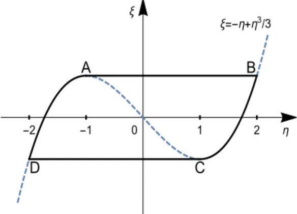
is a differential-algebraic system. This system does not define a dynamical system on the curve ξ = −η+η3/3 since on that curve there exist two points A(η = −1,ξ = 2/3) and C(η = 1,ξ = −2/3) which are so-called impass points: no solution of (1.5) can pass these points. LetB (D) be the point where the tangent to the curve ξ = −η+η3/3 at the point A (C) intersects the curve ξ =−η+η3/3 (see Figure1.1). We denote byZ0 the closed curve in the(η,ξ)-Liénard plane which consists of two segments of the curveξ =−η+η3/3 bounded by the points D,A and C,B and of two segments of the straight lines connecting the points A,BandD,C, respectively (see Figure1.1).
Using this closed curve Z0, D. A. Flanders and J. J. Stoker [2] constructed an annulus whose boundaries are crossed transversally by the trajectories of system (1.4) which contains the stable limit cycleΓε of system (1.4) for sufficiently small positiveε.
In what follows we present a new approach to establish the existence of a unique hyper- bolic limit cycleΓλof the van der Pol equation (1.1) for largeλwhich is based on a linear time scaling instead of applying the mentioned nonlinear Liénard transformation and on using an appropriate Dulac–Cherkas function.
A B
C D
η
-2 -1 1 2
ξ=-η+η3/3
0 ξ
Figure 1.1: Closed curveZ0.
2 Time scaled van der Pol system
We start with the van der Pol equation (1.1) and apply the time scaling σ = λ t for λ > 0.
Using the notationε=1/λ2we get the equation d2x
dσ2 + (x2−1)dx
dσ +εx=0 (2.1)
which is equivalent to the system dx
dσ =−y, dy
dσ =εx−(x2−1)y.
(2.2)
Settingε=0 in (2.2) we obtain the system dx
dσ =−y, dy
dσ =−(x2−1)y
(2.3)
which has the x-axis as invariant line consisting of equilibria. In the half-planes y > 0 and y<0, the trajectories of system (2.3) are determined by the differential equation
dy
dx = x2−1 and can be explicitly described by
y= x
3
3 −x+c, (2.4)
wherecis any constant.
Next we note the following properties of system (2.2).
Lemma 2.1. System(2.2)is invariant under the transformation x → −x,y→ −y.
This lemma implies that the phase portrait of (2.2) is symmetric with respect to the origin.
Lemma 2.2. The origin is the unique equilibrium of system(2.2), it is unstable forε>0.
Lemma 2.3. If system(2.2) has a limit cycleΓε, thenΓε must intersect the straight lines x = ±1in the lower and upper half-planes.
The proof of Lemma2.3is based on the Bendixson criterion and the location of the unique equilibrium.
For the sequel we denote byX(ε)the vector field defined by (2.2).
Lemma 2.4.
Ψ(x,y,ε)≡x2+ y
2
ε −1 (2.5)
is a Dulac–Cherkas function of system (2.2) in the phase plane forε>0.
Proof. For the functionΦdefined in (4.2) in the Appendix, we get from (2.5), (2.2) andκ=−2 Φ:= (gradΨ,X(ε)) +κΨdivX(ε)≡2(x2−1)2 ≥0 for(x,y,ε)∈R2×R+. (2.6) Since the setN, whereΦvanishes, consists of the two straight linesx=±1 which do not contain a closed curve, we get from Definition 4.1 and Remark 4.2 in the Appendix that Ψ represents a Dulac–Cherkas function for system (2.2) in the phase plane forε>0, q.e.d.
Forε >0, the setWε, whereΨ(x,y,ε)vanishes, consists of a unique oval, the ellipse Eε :=
(x,y)∈ R2: x2+ y
2
ε =1
. We denote byAε the open simply connected region bounded byEε.
Lemma 2.5. Forε>0,Eε is a curve without contact with the trajectories of system(2.1).
Proof. By Lemma4.3in the Appendix, any trajectory of system (2.2) which meets Eε intersects Eε transversally. It is easy to verify that any trajectory of system (2.2) which crosses Eε will leave the regionAε for increasingσ.
Lemma 2.6. System(2.2)has no limit cycle in Aε forε>0.
Proof. Ψ(x,y,ε)is negative for(x,y)∈ Aε. Thus, by Lemma4.4in the Appendix,|Ψ(x,y,ε)|−2 is a Dulac function in the simply connected regionAε forε>0 which implies that there is no limit cycle of system (2.2) in Aε forε>0.
Lemma 2.7. System(2.2)has at most one limit cycle forε>0.
Proof. For ε> 0, the set Wε consists of the unique ellipseEε. Thus, according to Theorem4.6 in the Appendix, system (2.2) has at most one limit cycle.
Lemma 2.8. If system (2.2) has a limit cycleΓε, thenΓε is hyperbolic and stable.
Proof. If system (2.2) has a limit cycle Γε, then by Lemma 2.6 and by Lemma 2.5, Γε must surround the ellipse Eε. Thus, we have Ψ > 0,κ = −2,Φ > 0 on Γε. Theorem 4.5 in the Appendix completes the proof.
We recall that for λ > 0 the van der Pol equation (1.1) and system (2.2) have the same phase portrait. Thus, the results above imply that the van der Pol equation has at most one limit cycleΓλ forλ6=0. In the following section we construct for sufficiently small εa closed curve Kε surrounding the ellipse Eε such that any trajectory of system (2.2) which meets Kε enters for increasingσthe doubly connected regionBε with the boundariesEε andKε.
3 Existence of a unique limit cycle Γ
εof system (2.2) for sufficiently small ε
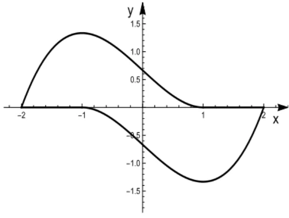
If we assume that there exists some positive number ε0 such that for 0 < ε < ε0 system (2.2) has a family{Γε}of limit cycles which are uniformly bounded, then the limit position ofΓεas εtends to zero is a bounded closed curve Γ0 symmetric with respect to the origin which can be described by means of solutions of system (2.3), that is, by segments of curves explicitly given by (2.4) and by segments of the invariant liney = 0 consisting of equilibria of system (2.3). SinceΓ0is a bounded smooth curve in the half-planesy≥0 andy≤0 and is symmetric with respect to the origin, we get forΓ0 in the upper half-plane the representation
y=−x+ x
3
3 + 2
3 for −2≤x≤1, y=0 for 1≤ x≤2.
The part in the half-planey≤0 is determined by the mentioned symmetry (see Figure3.1).
x y
-2 -1 1 2
-1.5 -1.0 -0.5 0.5 1.0 1.5
Figure 3.1: Closed curve Γ0.
We note thatΓ0consists of two heteroclinic orbits of system (2.3) connecting the equilibria (−2, 0) and (1, 0) in the upper half-plane and the equilibria (2, 0) and (−1, 0) in the lower half-plane, and of the two segments −2 ≤ x ≤ −1 and 1≤ x ≤ 2 of the x-axis consisting of equilibria of system (2.3).
In what follows, to given ε > 0 sufficiently small, we construct a closed curve Kε sur- rounding the ellipse Eε such that any trajectory of system (2.2) which meets Kε intersects Kε transversally. For the construction of the closed curve Kε we will take into account the following observations.
Remark 3.1. The amplitude of a possible limit cycle{Γε}of system (2.2) tends to 2 asεtends to zero.
Remark 3.2. Letε > 0. In the fourth quadrant(x <0,y > 0), the vector field X(ε)rotates in the positive sense (anti-clockwise) for increasing ε.
Remark 3.3. Letε>0. In the first quadrant, the vector field X(ε)rotates in the positive sense for decreasing ε.
Let P be the point (−2.2, 0) on the x-axis and let R be the point (2.2, 0) symmetric to P with respect to the origin. By Remark 3.1, there exists a sufficiently small positive number ε0
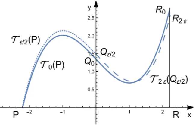
such that forε ∈ (0,ε0)any limit cycle Γε of system (2.2) intersects the x-axis in the intervals (−2.2, 0)and(0, 2.2). We denote byT0(P)the trajectory of system (2.3) in the upper half-plane havingP as ω-limit point. T0(P)intersects the y-axis at the point Q0 = (0,(2.2)3/3−2.2)≈ (0, 1.349)and the straight linex =2.2 at the point R0 = (2.2, 2[(2.2)3/3−2.2])≈ (2.2, 2.699). T0(P)is represented as solid curve in Figure3.2. LetTε/2(P)be the trajectory of system (2.2), whereε is replaced byε/2, in the fourth quadrant which passes the point P. For sufficiently smallε, it cuts the y-axis at the pointQε/2 which is near the point Q0. Tε/2(P)is represented as dotted curve in Figure3.2.
P R
Qε/2 Q0
R0 R2ε
2ε(Qε/2)
0(P)
ε/2(P)
x y
-2 -1 1 2
0.5 1.0 1.5 2.0 2.5
Figure 3.2: TrajectoriesT0(P),Tε/2(P)andT2ε(Qε/2)forε=0.08.
Now we denote byT2ε(Qε/2)the trajectory of system (2.2), whereεis replaced by 2ε, in the first quadrant which passes the pointQε/2. For sufficiently smallε,T2ε(Qε/2)is located near the trajectory T0(P)and intersects the straight line x = 2.2 at the point R2ε which is located near the pointR0. T2ε(Qε/2)is represented as dashed curve in Figure3.2.
According to Remark 3.2, any trajectory of system (2.2) (with the parameter ε), which meets the trajectoryTε/2(P)in the fourth quadrant, intersectsTε/2(P)transversally and enters for increasingσthe region ˜Dε/2 in the fourth quadrant bounded byTε/2(P), thex-axis and the y-axis (see Figure 3.3). By Remark 3.3, any trajectory of system (2.2) (with the parameter ε) which meets the trajectory T2ε(Qε/2) in the first quadrant intersects T2ε(Qε/2) transversally and enters for increasing σ the region ˜D2ε in the fist quadrant bounded by T2ε(Qε/2), the x-axis, they-axis and the straight linex =2.2 (see Figure3.3).
P R
Qε/2
R2ε
2ε(Qε/2)
˜
ε/2
˜
2ε
ε/2(P)
x y
-3 -2 -1 1 2 3
0.5 1.0 1.5 2.0 2.5
Figure 3.3: TrajectoriesTε/2(P)andT2ε(Qε/2)forε=0.08.
It can be easily verified that the trajectories of system (2.2) intersect the segment of the
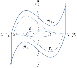
straight line x = 2.2 bounded by the points Rand R2ε transversally in the upper half-plane entering ˜D2ε for increasingσ. Since at the point R we have dy/dσ > 0, also the trajectory of system (2.2) passing R enters the region ˜D2ε for increasingσ. If we denote by ˜Kε,u the curve composed by the trajectoriesTε/2(P)andT2ε(Qε/2)and the segment of the straight linex=2.2 bounded by the points Rand R2ε, and introduce the set ˜Dε,u = D˜ε/2∪D˜2ε, then we have the following result: For sufficiently small ε, any trajectory of system (2.2) which meets the curve K˜ε,uenters for increasingσthe region ˜Dε,u. Exploiting the symmetry described in Lemma2.1 there exists a curve ˜Kε,l in the lower half-plane such that the closed curve ˜Kε = K˜ε,u∪K˜ε,l bounding the simply connecting region ˜Dε has the properties of the wanted closed curveKε. Figure3.4 shows the closed curves ˜Kε andEε bounding the annulus ˜Bε = D˜ε\ Aε containing the limit cycleΓε forε=0.08.
P R
ℰε
˜
ε,l
˜
ε,u
Γε
x y
-3 -2 -1 1 2 3
-3 -2 -1 1 2 3
Figure 3.4: Closed curves ˜Kε andEε together with the limit cycleΓε forε=0.08.
An improvement of the curve ˜Kε and consequently of the annulus ˜Bε containing the limit cycle Γε can be obtained as follows. Let T2ε(R) be the trajectory of system (2.2), where ε is replaced by 2ε, in the first quadrant starting at the point R. Since on the interval 0 < x <2.2 of thex-axis it holdsdy/dx=εx>0, the trajectoryT2ε(R)will intersect they-axis at the point Q2ε which is located between the origin and the point Qε/2. We denote by D2ε the region in the first quadrant bounded by the trajectoryT2ε(R), thex-axis and they-axis (see Figure3.5).
Using Remark 3.3, we can conclude as above that any trajectory of system (2.2) which meets T2ε(R)entersD2ε for increasingσ. For the following we denote byIε the interval on they-axis bounded by the points Qε/2 andQ2ε.
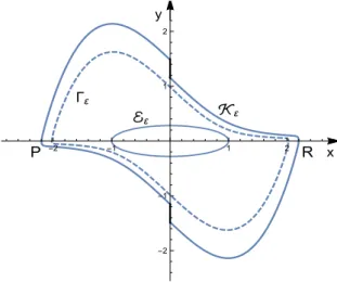
From (2.2) it follows that any trajectory of system (2.2) which meetsIε enters for increasing σ the region ˜Dε/2. Thus, we have the following result: There is a sufficiently small ε0 such that for ε ∈ (0,ε0) the trajectories Tε/2(P)and T2ε(R) and the interval Iε form a curve Kε,u which bounds in the upper half-plane the bounded region Dε,u = D˜ε/2∪ D2ε such that any trajectory of system (2.2) which meetsKε,u enters for increasingσ the regionDε,u. Exploiting the symmetry described in Lemma 2.1 there exists a curve Kε,l in the lower half-plane such thatKε =Kε,u∪ Kε,l forms the wanted closed curveKε. In Figure3.6the closed curvesKε and Eε are represented as solid curves which form the boundaries of the doubly connected region Bε which contains the unique limit cycleΓε (dashed curve) forε=0.08.
Summarizing our considerations we have the following results.
P R Qε/2
Q2ε
˜
ε/2
2ε
2ε(R) ℐε
ε/2(P)
x y
-2 -1 1 2
0.5 1.0 1.5 2.0
Figure 3.5: CurveKε,u =T2ε(R)∪ Iε∪ Tε/2(P)(R)forε=0.08.
P R
Γε
ε ℰε
x y
-2 -1 1 2
-2 -1 1 2
Figure 3.6: Closed curvesKε andEε and the limit cycleΓε forε=0.08.
Theorem 3.4. For sufficiently small positive ε, the closed curve Kε is a curve without contact for system(2.2), that is, any trajectory of system(2.2) which meets the curveKε crosses it transversally by entering the doubly connected regionBε for increasingσ.
Taking into account Lemma2.7and Lemma2.8 we get the following theorem from Theo- rem3.4.
Theorem 3.5. For sufficiently small positive ε, system(2.2)has a unique limit cycleΓε. This cycle is hyperbolic and stable and located in the regionBε.
4 Appendix
Consider the planar autonomous differential system dx
dt =P(x,y,λ), dy
dt =Q(x,y,λ) (4.1)
depending on a scalar parameterλ. LetΩbe some region inR2, let Λbe some interval and let X(λ) be the vector field defined by system (4.1). Suppose that P,Q : Ω×Λ → R are continuous in all variables and continuously differentiable in the first two variables.
Definition 4.1. A function Ψ : Ω×Λ → R with the same smoothness as P,Q is called a Dulac–Cherkas function of system (4.1) in Ω for λ ∈ Λ if there exists a real number κ 6= 0 such that
Φ:= (gradΨ,X(λ)) +κΨdivX(λ)>0(<0) for(x,y,λ)∈Ω×Λ. (4.2) Remark 4.2. Condition (4.2) can be relaxed by assuming that Φmay vanish inΩon a set N of measure zero, and that no closed curve of N is a limit cycle of (4.1).
In the theory of Dulac–Cherkas functions the set
Wλ :={(x,y)∈Ω:Ψ(x,y,λ) =0} (4.3) plays an important role. The following results can be found in [4].
Lemma 4.3. Any trajectory of system(4.1)which meetsWλ intersectsWλtransversally.
Lemma 4.4. Let Ω1 ⊂ Ω, Λ1 ⊂ Λ be such that Ψ(x,y,λ) is different from zero for (x,y,λ) ∈ Ω1×Λ1. Then|Ψ|κis a Dulac function inΩ1forλ∈Λ.
Theorem 4.5. LetΨ be a Dulac–Cherkas function of (4.1)inΩfor λ∈ Λ. Then any limit cycleΓλ
of (4.1)inΩis hyperbolic and its stability is determined by the sign of the expressionκΦΨonΓλ, it is stable (unstable) ifκΦΨis negative (positive) onΓλ
Theorem 4.6. Let Ωbe a p-connected region, letΨ be a Dulac–Cherkas function of (4.1) inΩsuch that the setWλ consists of s ovals inΩ. Then system(4.1)has at most p−1+s limit cycles inΩ.
References
[1] E. Fisher, The period and amplitude of the Van Der Pol limit cycle,J. Appl. Phys.25(1954), 273–274.MR0059436
[2] D. A. Flanders, J. J. Stoker, The limit case of relaxation oscillations, in: Studies in Non- linear Vibration Theory, Institute for Mathematics and Mechanics, New York University, 1946, pp. 51–64.MR0018780
[3] J.-M. Ginoux, C. Letellier, Van der Pol and the history of relaxation oscillations: toward the emergence of a concept,Chaos22(2012), 023120, 15 pp.MR3388537;https://doi.org/
10.1063/1.3670008
[4] A. A. Grin, K. R. Schneider, On some classes of limit cycles of planar dynamical sys- tems,Dyn. Contin. Discrete Impuls. Syst. Ser. A, Math. Anal.14(2007), 641–656.MR2354839 [5] A. Liénard, Étude des oscillations entretenues (in French), Revue générale de l’électricité
23(1928), 906–954.
[6] L. Perko,Differential equations and dynamical systems, Texts in Applied Mathematics, Vol. 7, Springer, 2001.https://doi.org/10.1007/978-1-4613-0003-8
[7] B. van der Pol, On relaxation-oscillations, The London, Edinburgh, and Dublin Philosoph- ical Magazine and Journal of Science, Ser. 7 2(1926), 978–992. https://doi.org/10.1080/
14786442608564127
[8] B.van derPol, J.van derMark, Le battement du cœur considéré comme oscillation de relaxation et un modèle électrique du cœur,L’Onde Électrique7(1928), 365–392.
[9] H. Yanagiwara, Maximum of the amplitude of the periodic solution of van der Pol’s equation,J. Sci. Hiroshima Univ. Ser. A-I Math.25(1961), 127–134.MR0147709