On the uniqueness of limit cycle for certain Liénard systems without symmetry
Dedicated to Professor László Hatvani on the occasion of his 75th birthday
Makoto Hayashi
1, Gabriele Villari
B2and Fabio Zanolin
31Department of Mathematics, College of Science and Technology, Nihon University, 7-24-1, Narashinodai, Funabashi, Chiba, 274-8501, Japan
2Dipartimento di Matematica e Informatica “U.Dini”, Università di Firenze, viale Morgagni 67/A, 50137 Firenze, Italy
3Dipartimento di Scienze Matematiche, Informatiche e Fisiche, Università di Udine, via delle Scienze 206, 33100 Udine, Italy
Received 29 June 2017, appeared 26 June 2018 Communicated by Jeff R. L. Webb
Abstract. The problem of the uniqueness of limit cycles for Liénard systems is investi- gated in connection with the properties of the functionF(x). Whenαandβ(α<0<β) are the unique nontrivial solutions of the equation F(x) = 0, necessary and sufficient conditions in order that all the possible limit cycles of the system intersect the lines x = α and x = β are given. Therefore, in view of classical results, the limit cycle is unique. Some examples are presented to show the applicability of our results in situations with lack of symmetry.
Keywords: Liénard system, uniqueness, limit cycles, invariant curves.
2010 Mathematics Subject Classification: 34C07, 34C25, 34C26, 34D20.
1 Introduction
In this paper we consider the well-known Liénard system
˙
x=y−F(x), y˙ =−g(x) (L)
with the aim to propose a necessary and sufficient condition in for the uniqueness of the limit cycle. Throughout the paper, our basic assumptions will be the following:
(C1) F(x)andg(x)are locally Lipschitz continuous functions;
(C2) F(0) =g(0) =0 andg(x)x>0 forx 6=0;
BCorresponding author.Email: villari@math.unifi.it
(C3) There existα andβ with α< 0 < βsuch that F(x) is strictly increasing forx ≤ αand x≥ βand, moreover,xF(x)<0 forx∈ (α,β)\ {0}.
We see under the above assumptions that the uniqueness of solutions of system (L) for initial value problems is guaranteed and the only equilibrium point (0, 0) is unstable. This sys- tem has been widely investigated in the literature (for instance see [5] or [18]) and plays an important role in the qualitative analysis of planar ODEs and applications.
As a starting point, we recall the classical uniqueness results due to Liénard [8], Levinson–
Smith [7] and Sansone [10] from which the following result can be deduced.
Proposition 1.1. Under the conditions(C1),(C2)and(C3)there is at most a limit cycle intersecting both the lines x= αand x= β.
In view of Proposition1.1, it can be useful to introduce the following terminology.
Definition 1.2. System (L) has the property (A)if all its limit cycles intersect the lines x = α andx=β.
In the above quoted papers, the authors assume some symmetry conditions ensuring that property (A) is fulfilled. If no symmetry condition onF(x)andg(x)is assumed, it is necessary to produce sufficient conditions for the validity of (A) and hence for the uniqueness. In this light, sufficient conditions for property (A) were proposed by several researchers (cf. [2,6,11]
and the recent paper [15]). For related results, in a more general environment, see also [1,9,17].
In [6], the relation between the magnitude ofF(x)and the unique existence of a limit cycle of system (L) has been investigated and the following condition was introduced.
(C4)
G(α)>G(β), ∃x2∈ (0,β] such that 1
2F(x2)2+G(β)< G(α) or
G(α)≤G(β), ∃x1∈[α, 0) such that 1
2F(x1)2+G(x1)≥G(β), whereG(x) =Rx
0 g(ξ)dξ.
Proposition 1.3 ([6]). Under the conditions (C1), (C2), (C3) and (C4), property (A) holds and therefore system(L)has at most one limit cycle which is stable.
The case in which system (L) does not satisfy condition (C4) has been recently investigated in [15]. Further results in this direction will be presented in this paper. In particular, in Section2we give necessary and sufficient conditions in this direction. Finally, in Section4we present some concrete examples which involve new applications and show the effectiveness of this approach.
It is worth to note that in the same context, but with a different approach, in a very recent paper [16], the monotonicity assumption on F(x), and therefore the sign assumption on f(x), were strongly relaxed.
2 Main results
As observed in the previous section, the values of the function G(x) at the points α and β play a crucial role. For this reason, we investigate in detail the situation. IfG(α) = G(β), we
note that there exists x1 = αsatisfying the condition (C4) (see also Example 4.1) and hence Proposition1.3applies. So we focus our attention to the case
G(α)≤ G(β), (2.1)
the case G(β) < G(α) being treated in a symmetric way. Therefore, from now on, we take (2.1) as a basic assumption for the rest of the paper.
For x ∈ [α, 0] we consider the points in which the functionΦ(x) := F(x)2+2G(x)takes its maximum and letabe the maximum of such points. In other words,
a =maxn
x ∈[α, 0]|Φ(x) = max
ξ∈[α,0][F(ξ)2+2G(ξ)]o. Clearly,a <0 and, by definition,
F(a)2+2G(a) = max
ξ∈[α,0]Φ(ξ)≥ Φ(α) =F(α)2+2G(α) =2G(α). (2.2) In virtue of (2.1) and (2.2), only the following two cases can occur and so they will be taken into consideration:
Case 1. F(a)2+2G(a)≥2G(β),
Case 2. 2G(α)≤F(a)2+2G(a)<2G(β), The following result holds.
Theorem 2.1 (Case 1). Let F(a)2+2G(a) ≥ 2G(β)or G(α) = G(β). If system (L) satisfies the conditions (C1),(C2),(C3), then the system satisfies the property(A)and therefore it has at most one limit cycle.
Remark 2.2. The case 1 can be rewritten in the following form
xmax∈[α,0]
n
F(x)2+2G(x)o≥2G(β).
We consider now Case 2 or and lety(x)be the solution of system (L) with y(0) =
q
F(a)2+2G(a). (2.3)
Let alsoγ∈ (0,β)be such that 2G(γ) =2G(β)−y(0)2, that is
F(a)2+2G(a) =2G(β)−2G(γ). (2.4) In this case, the following result holds.
Theorem 2.3(Case 2). Assume that system(L)satisfies the conditions(C1),(C2),(C3)and F(a)2+ 2G(a)<2G(β).Then the system satisfies the property(A)and therefore it has at most one limit cycle if and only if there exists c∈ (γ,β)such that
(C5) y(0) = q
2(G(β)−G(c)) +
Z c
0
g(x) y(x)−F(x)dx.
Condition (C5), even if necessary and sufficient, is of implicit type because it require the knowledge of the solutiony(x). Accordingly, it may be useful to state some corollaries which guarantee that such a condition is automatically satisfied. Taking into account that y(x)>0, g(x)>0 andF(x)<0 for all x∈ (0,c), we have the following consequence of Theorem2.3
Corollary 2.4. Under the conditions in Theorem2.4if there exists c∈ (γ,β)satisfying the inequality (C6) y(0)≥q2(G(β)−G(c)) +
Z c
0
g(x) y(0)−F(x)dx,
then the system satisfies the property(A)and therefore it has at most one limit cycle.
Remark 2.5. We just observe that if, instead of (2.1), we assume the dual hypothesis G(α)>
G(β), the condition (C6) will be replaced by (C6)∗ y(0)≤
q
2(G(α)−G(c0)) +
Z c
0
0
g(x) y(0)−F(x)dx,
where c0 ∈ (α,γ0), γ0 < 0 and 2G(γ0) = 2G(α)−y(0)2. This inequality will be used in Example4.3.
As previously observed, the presented results guarantee the existence of at most one limit cycle. In order to obtain the existence, it is necessary to add some other assumption, which will guarantee that the orbits of the systems will be ultimately bounded and the classical Poincaré–Bendixson theorem can be applied. Typical condition make use of assumptions on Fand/or Gat infinity. In this light, following [3,5,12,14], we have the following theorem.
Theorem 2.6. If system(L)satisfies the conditions in Theorem2.1, or Corollary2.4, and (C7) lim sup
x→±∞
n
G(x)±F(x)o= +∞,
then it has a unique limit cycle which is stable and hyperbolic.
For condition (C7), see [12].
3 Proofs of the results
At first we consider Theorem 2.1, which is essentially the result in [6] and also recalled in Proposition1.3. We give quick details for the sake of completeness.
Let F(a)2+2G(a) ≥ 2G(β). The case G(α) = G(β) is well known (see [3,6,10]). We introduce the energy function
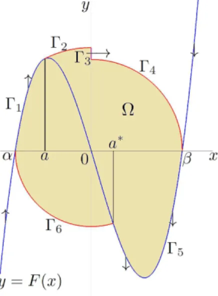
V(x,y):= (1/2)y2+G(x) and define the plane curveΓconstructed by six curves as follows.
Γ
Γ1:y= F(x) forx ∈[α,a]
Γ2:V(x,y) = (1/2)F(a)2+G(a) forx∈[a, 0], y≥0 Γ3:x =0, p
2G(β)≤ y≤pF(a)2+2G(a) Γ4:V(x,y) =G(β) forx∈ [0,β], y≥0 Γ5:y= F(x) forx ∈[a∗,β]
Γ6:V(x,y) =G(α) forx ∈[α,a∗], y≤0,
where a∗ is a positive number satisfying the equationV(x,F(x)) = G(α). Such construction may be found in [6]. See Figure3.1below. Keep following [6], one can check that the domain
Figure 3.1: (Case 1). For the example considered in the figure, we have cho- sen g(x) = x and F(x) = k(x+ 52)(x−3), with k = 9/20. The shadowed region represents the set Ω. We have α = −5/2, β = 3 and we can estimate a ; −1.537662135 and a∗ ; .7246695283. We also find that F(a)2+2G(a) ; 11.49431131>2G(β) =9, so that we are in the situation of [6] and Theorem2.1 applies.
Ωsurrounded by the closed curveΓand including the equilibrium pointOhas the vector field pointing outside at the boundary. Moreover, it is proved that no limit cycles of the system can exist in the interior of Ω. Thus, any possible limit cycle must lie outside Ω, and therefore it will intersect the linesx =αandx= β. Hence the property (A) is fulfilled and this completes the proof of Theorem2.1.
For the proof of Theorem2.3 it is useful to premise the following statement whose trivial proof is omitted.
Lemma 3.1. Let p
2(G(α)) ≤ y(0) ≤ p2(G(β)),and γ as in(2.3) and(2.4). The orbit starting from(0,y(0))intersects the plane curve y= p2(G(β)−G(x))if and only if there exists c∈ (γ,β] satisfying the equality y(c) =p2(G(β)−G(c)).
Now we are in position to give a proof for Theorem2.3.
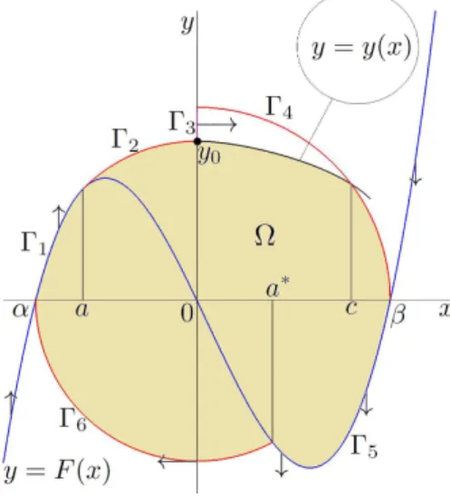
Lety(0) =pF(a)2+2G(a)as in (2.3). If the solution orbity=y(x)starting from(0,y(0)) intersects the plane curve Γ4 on the boundary of the domain Ω at x ∈ (c,β), then we have from Lemma3.1
y(0) =y(c)−
Z c
0
dy(x) dx =
q
2(G(β)−G(c))−
Z c
0
−g(x) y(x)−F(x)dx
and hence (C5). Moreover, since the solution orbit cannot return in Ω, it will intersect the line x = β. On the other hand, if we start from a point on the segment Γ3, namelyx = 0 and pF(a)2+2G(a)≤ y≤p2G(β)), back in time, the orbit must have intersected thex=αand, forward in time, it will stay above the the previously considered orbit (x,y(x)) x = β and therefore it will intersect x= β, giving the desired property (A). See Figure3.2
The converse is trivial.
We note that ify(0) =p2G(α), then the two curvesΓ1andΓ2are replaced by the curveC∗ which is the energy levelV(x,y) =G(α), forx ∈[α, 0], y≥0.
Figure 3.2: (Case 2). For the example considered in the figure, we have cho- sen g(x) = x and F(x) = k(x+ 52)(x−3), with k = 7/25. The shadowed region represents the part of the set Ω bounded by the orbit path passing through(0,y0)with y0 = y(0). We haveα= −5/2,β = 3 and we can estimate a ; −1.769233452 and a∗ ; 1.175057813. We also find that F(a)2+2G(a) ; 6.111041847<2G(β) =9 and in this case Theorem2.1does not apply.
For a previous step in this direction, see [15] where only a sufficient condition was given, whereRc
0 g(x)
y(x)−F(x)dxwas replaced byRc 0
g(x)
−F(x)dx.
Finally, we prove Theorem 2.6. We observe that, recently, M. Cioni and G. Villari ([3]) have proved the existence of the limit cycles for the system under the condition (C7). Other conditions may be found in the literature and appear, for instance, in the references of the above mentioned paper. Consequently, putting together the existence results coming from (C7) and the uniqueness of the limit cycle following from Theorem2.1 and Corollary2.4, we get the thesis.
4 Examples
We shall present concrete systems for system (L) as applications of our results. The first one is very elementary and classic, while the other two show the concrete applicability of our results.
Example 4.1. We consider the well-known Van der Pol systemF(x) =λ 13x3−x
andg(x) = x. It is classical fact that such system has exactly one limit cycle. It is worth to note that, among the others, there is a very elegant uniqueness proof due to Massera (see, for instance, [13] and the references therein). However, it is possible to get the same result, just observing that, due to the symmetry properties,G(α) =G(β).
Example 4.2. Consider system (L) withF(x) =√
3x(x+1)(x−3)andg(x) =x. By the choice ofgandFwe have thatG(x) =x2/2 andα=−1,β=3. The value of the constantafor which
we obtain the maximum of the function F(x)2+2G(x)forx∈[α, 0]is
a;−.5646076839 (4.1)
for which we have
F(a)2+2G(a);2.622343392 and y(0);1.619365120.
Now we observe that, if we wish to apply Corollary 2.4, we can start also from a constant a which is not the optimal one as in (2.2) (which, for our case, would be the one computed in (4.1)). Indeed, if we chose another constant a ∈ (α, 0), we will produce a lower value with respect to the optimal choice of y(0). However, if we are able to get (C6) satisfied for a lower value ofy(0), then (C6) also will hold for the optimal one.
To show how our result can be applied even if we not use the optimal value of the constant agiven above, let us choosea =−1/2 and observe that
F(a)2+2G(a) = 163
64 =2.546875<2G(β) =9.
As a next step, we can computey(0)using (2.3), as y(0) =
q
F(a)2+2G(a) =
√413
8 ;1.595893166 and also γ∈ (0, 3) = (0,β)using (2.4), from which we have
γ= q
2G(β)−2G(a)−F(a)2=
√ 413
8 ;2.540300179.
After these preliminaries, we can easily find (with a little help of some numerical integration), that there existsc∈ (γ,β]satisfying the inequality (C6) in Corollary2.4. In fact, taking
c= 14
5 =2.8∈ (γ,β), we have
K := q
2(G(β)−G(c)) +
Z c
0
g(x) y(0)−F(x)dx
= 1 5
√ 29+
Z 14/5
0
√ x
413
8 −√
3x(x+1)(x−3)dx;1.519184294.
Thus we have find thaty(0)>K and Corollary2.4applies, ensuring that the system
˙
x=y−√
3x(x+1)(x−3), y˙ =−x has a unique limit cycle. A numerical simulation is shown in Figure4.1
We point out that the condition (C4) cannot be applied to this example since G(α)<G(β) and 2G(α)< max
α≤x≤0F(x)2+2G(x)<2G(β)
This example shows that in this case Theorem 2.1 and the results in [6] cannot be applied, while Corollary2.4finds its applicability.
Figure 4.1: Phase-portrait for Example4.2, with the unique limit cycle.
Example 4.3(Duff and Levinson [4]). The following system was studied in [6] as an example for the unique existence of the limit cycle with the property (A).
˙
x =y−λ 64
35πx7−112
5πx5+196 3πx3−C
2x2− 36 πx
, y˙ =−x (DL)
This example is crucial, because in the fundamental paper [4] it was proved that the system has three limit cycles when when λ is sufficiently small and C is large. The importance of this result lies on the fact that before the work of Duff and Levinson it was believed that the condition thatF(x)has three zeros α<0< βwas actually ensuring the uniqueness.
LetC=47. In [6], it was proved that the system has the property (A) ifλ≥2.86896. Slight different examples appear also in [3,15].
In virtue of Corollary2.4and Remark2.5the estimate obtained [6] in is now replaced and improved by the following statement.
Proposition 4.4. System (DL) has the property (A) and hence a unique limit cycle if C = 47, for everyλ≥0.862.
Proof. In fact, solving the equation F(x) = 0, we have α ; −3.18941, β ; 0.3715. Moreover g(x) =x.
To prove(C6)∗, namely y(0)≤ −
q
2(G(α)−G(c0)) +
Z c
0
0
g(x)
y(0)−λF(x)dx,
we setλ=0.862 and choose c0= −3.18. Then, fory(0) =−p2G(β) =−β, we have
−0.3715≤ − q
α2−c02+
Z c0
0
x
−β−λF(x)dx
;−0.244818602−0.126575= −0.371393602, thus proving(C6)∗.
Acknowledgments
The authors gratefully thanks the referee for the useful comments which led to an improved version of the paper.
The work of G. V. and F. Z. has been performed under the auspices of the Gruppo Nazionale per I’Analisi Matematica, la Probabilità e le loro Applicazioni (GNAMPA) of the Istituto Nazionale di Alta Matematica.
References
[1] T. Carletti, Uniqueness of limit cycles for a class of planar vector fields, Qual. Theory Dyn. Syst.6(2005), 31–43.https://doi.org/10.1007/BF02972666;MR2273488
[2] T. Carletti, G. Villari, A note on existence and uniqueness of limit cycles for Lié- nard systems,J. Math. Anal. Appl.307(2005), 763–773.https://doi.org/10.1016/j.jmaa.
2005.01.054;MR2142459
[3] M. Cioni, G. Villari, An extension of Dragilev’s theorem for the existence of periodic solution of the Liénard equation, Nonlinear Anal.127(2015), 55–70.https://doi.org/10.
1016/j.na.2015.06.026;MR3392358
[4] G. F. Duff, N. Levinson, On the non-uniqueness of periodic solutions for an asymmetric Liénard equation, Quart. Appl. Math. 10(1952), 86–88. https://doi.org/10.1090/qam/
46511;MR0046511
[5] J. Graef, On the generalized Liénard equation with negative damping,J. Differential Equa- tions12(1972), 34–62.https://doi.org/10.1016/0022-0396(72)90004-6;MR0328200 [6] M. Hayashi, On the uniqueness of the closed orbit of the Liénard system, Math. Japon.
46(1997), No. 3, 371–376.MR1487283
[7] N. Levinson, O. K. Smith, A general equation for relaxation oscillations, Duke Math. J.
9(1942), 382–403.MR0006792
[8] A. Liénard, Étude des oscillations entretenues (in French), Revue générale de l’Electricité, 23(1928), pp. 901–912, 946–954.
[9] M. Sabatini, G. Villari, Limit cycle uniqueness for a class of planar dynamical systems, Appl. Math. Lett. 19(2006), 1180–1184. https://doi.org/10.1016/j.aml.2005.09.017;
MR2250355
[10] G. Sansone, Sopra l’equazione di A. Liénard delle oscillazioni di rilassamento (in Ital- ian), Ann. Mat. Pura Appl. (4)28(1949), 153–181.https://doi.org/10.1007/BF02411124;
MR0037430
[11] G. Villari, Some remarks on the uniqueness of the periodic solutions for Liénard’s equation, Boll. Un. Mat. Ital. C (6)4(1985), 173–182.MR805212
[12] G. Villari, On the qualitative behaviour of solutions of Liénard equation, J. Dif- ferential Equations67(1987), 269–277. https://doi.org/10.1016/0022-0396(87)90150-1;
MR879697
[13] G. Villari, An improvement of Massera’s theorem for the existence and uniqueness of a periodic solution for the Liénard equation,Rend. Istit. Mat. Univ. Trieste44(2012), 187–195.
MR3019560
[14] G. Villari, F. Zanolin, On a dynamical system in the Liénard plane. Necessary and suf- ficient conditions for the intersection with the vertical isocline and applications, Funkcial.
Ekvac.33(1990), 19–38.MR1065466
[15] G. Villari, F. Zanolin, On the uniqueness of the limit cycle for the Liénard equation, via comparison method for the energy level curves, Dynam. Systems Appl.25(2016), 321–334.
MR3615770
[16] G. Villari, F. Zanolin, On the uniqueness of the limit cycle for the Liénard equation with f(x) not sign-definite, Appl. Math. Lett. 76(2018), 208–214. https://doi.org/10.
1016/j.aml.2017.09.004;MR3713518
[17] D. Xiao, Z. Zhang, On the uniqueness and nonexistence of limit cycles for predator–prey systems, Nonlinearity 16(2003), 1185–1201.https://doi.org/10.1088/0951-7715/16/3/
321;MR1975802
[18] Z. F. Zhang, T. R. Ding, W. Z. Huang, Z. X. Dong, Qualitative theory of differen- tial equations, Translations of Mathematical Monographs, Vol. 102, AMS, Providence, 1992.
MR1175631