DATABASE MANAGEMENT SYSTEMS
Radványi, Tibor
DATABASE MANAGEMENT SYSTEMS
Radványi, Tibor Publication date 2014
Szerzői jog © 2014 Hallgatói Információs Központ Copyright 2014, Felhasználási feltételek
Tartalom
1. DATABASE MANAGEMENT SYSTEMS ... 1
1. Introduction ... 1
2. Basic Elements ... 2
2.1. Data and Information ... 2
2.2. Database ... 3
2.3. Database Management System (DBMS) ... 4
2.3.1. Local database ... 5
2.3.2. File – server architecture ... 5
2.3.3. Client – server architecture ... 6
2.3.4. Multi-Tier ... 8
2.3.5. Thin client ... 9
2.4. Basic structures ... 9
3. Improvement of data models ... 9
3.1. Hierarchical ... 10
3.2. Network Data Model ... 11
3.3. Relational ... 11
4. Database planning and its contrivances ... 15
4.1. Main steps of database designing ... 16
4.2. Normalisation ... 17
4.2.1. Normal Forms: ... 17
4.2.2. Dependences ... 17
4.2.3. Relation key ... 18
4.3. Data model mistakes ... 19
4.4. Stopping the redundancy ... 21
4.4.1. Normal forms: ... 21
4.4.2. Third normal form: ... 24
4.4.3. Boyce/Codd normal form (BCNF) ... 25
4.5. The relation‘s third normal form and the decomposition of the Boyce/Codd normal form 25 4.5.1. Fourth normal form (4NF) ... 25
4.5.2. Fifth normal form (5NF) ... 25
4.6. Physical designing ... 26
4.7. Supporting the design with software ... 26
4.7.1. Designing requirements: ... 26
4.7.2. Design of the database, the database tables and their fields: ... 26
4.8. The MySQL WorkBench ... 27
4.9. Operations of relational algebra ... 31
4.10. Tasks ... 35
4.11. Connecting Tables ... 54
4.12. Views and Indexes ... 77
4.13. Constraints, integrity rules, triggers ... 83
4.14. Tasks ... 91
4.15. Basics of PL/SQL ... 94
4.15.1. Character set ... 94
4.15.2. Lexical units ... 95
4.15.3. Symbolic names ... 95
4.15.4. Reserved words ... 96
4.15.5. Literals ... 96
4.15.6. Label ... 96
4.15.7. Variable ... 96
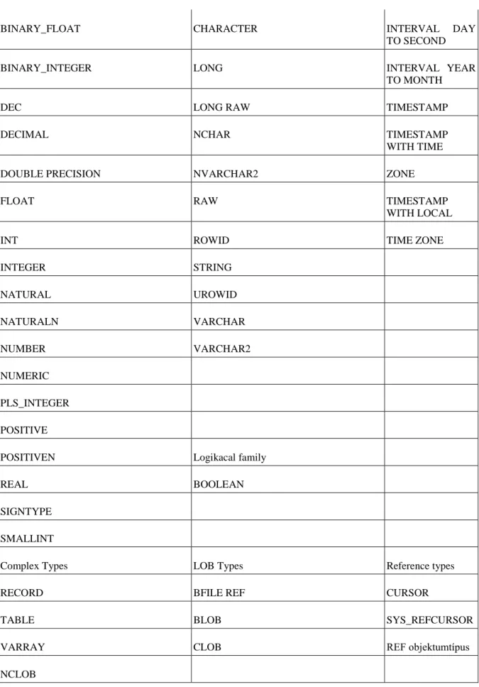
4.15.8. Simple and complex types ... 97
4.15.9. NUMBER type ... 98
4.15.10. Character family ... 99
4.15.11. Date/interval types ... 100
4.15.12. Logical type ... 100
4.15.13. Record type ... 100
4.16. Mixed Tasks ... 107
5. Language Reference of SQL ... 113
5.1. Elements of DDL ... 113
5.1.1. Create schemes, the creat ... 113
5.1.2. Changed the schema elements, the alter ... 114
5.2. .Elements of the DML ... 116
5.2.1. New data entries, insert the command ... 116
5.2.2. .Delete data, the delete ... 117
5.3. Queries and the QL ... 119
5.3.1. The base of the select command ... 119
5.3.2. Aggregation queries, the usage of group by and having, and arrangement 125 5.3.3. Connecting Tables ... 128
5.3.4. Embedded queries ... 131
5.4. Tasks ... 133
6. Views and Indexes ... 151
6.1. View ... 151
6.1.1. Modifiable view tables ... 152
6.1.2. Structural terms of modifiability: ... 152
6.1.3. Deleting a view table ... 152
6.1.4. Consequently, let‘s look through the advantages of view tables: ... 152
6.2. Indexes ... 153
6.2.1. Sparse indexes ... 153
6.2.2. Searching ... 153
6.2.3. Insertion ... 153
6.2.4. Deleting ... 154
6.2.5. Modifying: ... 154
6.2.6. B*-trees as multilevel sparse indexes ... 154
6.2.7. Searching: ... 154
6.2.8. Insertion: ... 155
6.2.9. Delete: ... 155
6.2.10. Modification: ... 155
6.3. Dense indexes: ... 155
7. Constraints, integrity rules, triggers ... 156
7.1. ... 156
7.1.1. Keys ... 156
7.1.2. Referential integrity constraint ... 158
7.2. ... 158
7.2.1. Constraints for attribute values ... 159
7.3. ... 159
7.3.1. Standalone assertions ... 159
7.4. ... 159
7.4.1. Modifying constraints ... 159
8. Triggers: (Oracle 10g) ... 160
8.1. Triggers could triggered by: ... 160
8.2. ... 160
8.2.1. We use them in the following cases: ... 160
8.3. ... 161
8.3.1. Row-level trigger: ... 161
8.4. ... 161
8.4.1. Statement-level trigger ... 161
8.5. ... 162
8.5.1. Before and After triggers: ... 162
8.6. ... 163
8.6.1. Instead of trigger ... 163
8.7. ... 163
8.7.1. System triggers ... 163
8.8. ... 163
8.8.1. Creating Triggers ... 163
8.9. ... 164
8.9.1. How triggers work: ... 164
8.10. Tasks ... 165
9. Basics of PL/SQL ... 167
9.1. Basic elements of PL/SQL ... 167
9.1.1. Character set ... 167
9.1.2. Lexical units ... 168
9.1.3. Symbolic names ... 168
9.1.4. Reserved words ... 169
9.1.5. Identifiers with quotation marks: ... 169
9.1.6. Literals ... 169
9.1.7. Label ... 169
9.1.8. Simple and complex types ... 170
9.1.9. NUMBER type ... 171
9.1.10. Character family ... 172
9.1.11. ROWID, UROWID Types ... 173
9.1.12. Date/interval types ... 173
9.1.13. Logical type ... 173
9.1.14. Record type ... 173
9.2. Programming structures ... 175
9.2.1. The CASE statement ... 176
9.2.2. Loops ... 177
9.2.3. Base loop ... 177
9.2.4. While loop ... 178
9.2.5. FOR loop ... 179
9.2.6. The EXIT statement ... 179
10. Mixed Tasks ... 180
1. fejezet - DATABASE
MANAGEMENT SYSTEMS
Dr. Radványi Tibor 2014.01.13
1. Introduction
Data and information. These two things became leading factors through the past 50 years and during the 20th and 21th century as these concepts play a significant part of our everyday life. As in our society the role of the information is being valorised, we are getting more and more pieces of information. We are continuously bombed with information from the outside world: we get the news from the television, radio, and newspapers and we are being informed about the latest happenings from the fellow human beings all day long. Of course we try to sort out and concentrate on the most important ones from the quarry of information. It is especially relevant as it seems to be impossible to memorize all the pieces of information. Sometimes we simply can‘t memorize or wouldn‘t like to memorize them. Accordingly we have to find another way of recording information instead of keeping them in mind. As the old Latin tag has it - verba volant, scripta manent – spoken words fly away, written ones remain. In addition everybody has a share in reaching the recorded information in a fast and easy way.
Information equals power as the proverb says. And actually it is right. I‘m sure that explaining the importance of keeping our bank card‘s details at an appropriate place is not necessary. That‘s why it would be advisable to find the safest way of storing information. We should find the best method to be able to reach them in an easy, simple, and fast way.
So, we can easily admit that students should acquire this bunch of learning during their primary and secondary school studies (and of course during their lives). According to the National Curriculum‘s assumption in the field of developments, our educators should pay more attention on teaching the basic computer skills. Indeed, in this field the number of the lessons was raised. Because of the above-mentioned reasons cognition of databases and database management systems play a particularly important role. Moreover, it is useful for students (and of course for everyone) to keep up with the changes, aims, and reformations of the developments of informatics.
Furthermore the number of the people working with informatics and the level of their qualification is rising mightily. Let‘s keep up with both aspects as the claim to well-qualified professionals is getting higher and higher.
One of the computer science‘s main characteristics is the following: more and more users use data, stored on more and more computers. Ready and applied software systems have to deal with always rising amount of data.
In our everyday life we meet the usage of computer information systems more and more often. Computer information systems are frequently used in factories to control different operations like production, finance, the staff‘s work, storage, and economization. We can mention some fields of usage in every part of our lives:
1. Commercialism: registration of the stock 2. Civil service: taxation
3. Hygiene: registration of the sick
4. Transport: system of reservations, timetables 5. Engineering: designer systems
6. Education: student‘s registration
All of them have a common feature: they all maintain a large data set, there are complicated relations between the data items, and these data sets have to be retained for a long period of time.
Of course there are other main features of these systems, but there are requirements which have to be fulfilled:
1. Maintaining a large amount of data
2. Supporting more users to be able to access at the same time 3. Keeping integrity
4. Protection
5. Effective software development
2. Basic Elements
The first databases were established from file control services in the early ‗60s. They were extensive and expensive program systems which were run on large sized computers. The first significant usage fields of them were the systems in which huge pieces of data were stored, including numerous queries and modifies. For example: Companies‘ card indexes, banks‘ systems, flight booking systems.
Since 1970, the publication of Ted Codd‘s article, in which he suggested that the database management systems should present the data in tables for the user, database management systems have appreciably changed.
The difference to the previously used systems is that in the relational system the user doesn‘t have to deal with the structure of data storage, as queries can be expressed with such a high-level language, that its usage highly increases the efficiency of database programmers.
In this model there are no highlighted data, so the features registered about the items of the set are equal. This way the system can be used more flexible as the search strings can be drawn optionally.
The first corporation, selling both database systems supporting databases before relational models and systems supporting relational models, was IBM.
Lately database systems based on relational models are as current computer tools as word processors or spreadsheet programmes used to be.
2.1. Data and Information
Information plays the main role in our world. If we wanted to feature our society with an attributive structure, it would be evident to name it information society. I wonder if we clearly know what information means. A totally acceptable definition hasn‘t been found yet, although every speciality dealing with information has formed its entity, featured with marks being important in their point of view; named information.
Information is the experienced, sensed, and understood data which is useful and new for the taker, who construes it according to their previous store of learning.
Data means the appearance of a fact which we can record, store, modify, and send on. The conception of data is not an exact idea. In the point of view of database designing, data is the meaningless series of signs from which we can earn information after processing.
Although till then it is just a meaningless series of signs. If we collect some data and we store them in a given place including the connections between them, we have created a database:
E.g.: the medical cards of the sick, details of cars at the police, notes of a telephone directory.
2.2. Database
A database is the whole bulk of integrated and logically connected pieces of information; the system of data and connections between them; stored abreast. To be able to work with our database effectively deliberate designing is essetial.
The concept of database system consists of the databases, the computer resources, moreover, in a wider sense, the database-administrators, who are the ones who put through the designing and programming of the database.
2.3. Database Management System (DBMS)
The database is a kind of data collection. It stores data, which is in connection with the given task, orderly. The access to the data is also taken care of by the database. Besides, it guarantees the protection of the data, and also protects the integration of the data.
The management of the data was also made easier by database management systems.
The ANSI/SPARC model shows the connection between the user and of the physically stored data on the computer‘s mass storage.
We distinguish three levels, based on that:
• Outer level, alias user view, which examines the data from user‘s point of view.
• Conceptual level, which includes all of the user views. In this level the database is given with logical schema.
• Inner level, alias physical level, it means the actual presentation of the data on the current computer.
When we talk about ANSI/SPARC model it is important to mention two things. These are the logical data independence and the physical independence. Physical independence means that if we change anything in the inner level it will not effect anything on the logical schema.
So, we will not have to perform changes on them. If any changes occur in the storage of data it will have no effect on the upper levels. The logical data independence is data independence between outer level and conceptual level.
Those program systems which are responsible for guaranteeing access to the database are called database management systems. Furthermore, the database management system takes care of the tasks of the inner maintenance of the database such as
• Create database
• Defining the content of the database
• Data storage
• Querying data
• Data protection
• Data encryption
• Access rights management
• Physical organization of the data structure
We must keep in mind how the architecture of the database has changed. Furthermore, it is also important how we can put these together. It is very important for the programmers, because they are in a situation where they have to choose what they are going to working with after they have got the order. Because, those are not good programmers or software developers who can only use one database management system, or those who can write programs only in one programming language. That is the expectation of an elementary school. If you get a task it is good if you can decide which route is the one you have to start. What database manager you should use and in which programming language you are going to write your program. Of course, one could not say that know all of the existing programming languages by heart. We will talk about two or three of them. But everybody knows who have tried to make web pages that it might not be a good idea to start a webpage development for example with an aspx.net. In one hand, it is possible in the case of a bigger task that aspx.net is good. On the other hand, one could possibly do a smaller task with html code without putting any dynamism in it, or maybe in php the things could be done easier. These are specific things. Returning to the database architectures, now the question is in which environment certain database managers can do good performance.
Because, it is not true that every database manager can satisfy our needs in all environments.
2.3.1. Local database
The first such architectural level is the local database: these are the ―best‖. It contains a computer, a database, a user, nobody has any problem. The story started sometime around 1980s. Database managers have appeared in the computers. It was the world of the dBase, which was based on the Dos. (From the beginning, DOS did not allow multi users and to run on more paths.) Back then there were no such problems as web collusion or concurrent access. Such database were dBase 3, 4, 5, the developed version of this were Paradox 4, 5, 7, which had more stable data table management, but in return we have got a more damageable index table. The following things were true for all of them: one database - one file; one index - one file; one descriptor table - one file; one check term for a table – one file. If we had a database with 100 tables then there was created 100 files in a directory. These were managed by a database management engine. It worked on file levels, moved bytes and managed blocks. As it worked on file level it was damageable. There were a lot of files. So, there were already a big possibility of damage and big possibility of delete on the level of the operation system. If there was a power shortage, it was necessary to call the programmer, because the whole system has turned upside down.
Something for something. I always say that these are dangerous systems, especially, if we do not use them in local database system. Nowadays, it would be very hard to use local database. The MS Access is also belonging to there. It is only more modern, because of the fact that all of the tools, data and descriptive tools are stored in the same file. From there it knows it knows the same as Paradox or dBase. It could become very damageable if we want to use under bigger stress. They are perfect for teaching (ECDL, for final examination). The LibreOffice also has the Base database. That is similar to Access. It is also free, and it is good for familiarization and teaching. These database managers have limits. In a traffic table the numbers of records are continuously growing. It can easily reach the quantity of 100000. It may seem to be more, however if somebody write a system that is also being used, it turns out to be few. One could not say that up to 100000 it works well, but at 100001 the whole system fall apart. It works well two to three hundred-thousand, but after it more and more error occurs. The system is start slowing down and index damages are coming up. So, the efficiency of the local, file-based systems has the volume of 100000. If we know that and if we know the kind of work they want to give us then it is not a problem to use them. if we have to make a database for Marika‘s flower shop where she would put her data. For example, she wants to store that she has got 10 tulips and 30 roses and that she has sold 9 tulips and 34 roses, and nothing more. In this case the Access is more than enough for her. Don‘t try to convince her that she needs Oracle.
2.3.2. File – server architecture
Of course, the world has developed. There is cable so we can connect any number of computers. But the problem was that the database management was young at that time. So, they have developed this wonderful file – server architecture. I have to mention it in parentheses that although the use of the Novell server is not exclusive, but its best time was then. That hasn‘t been so long, about 15 years. But in the information technology that had been a long time. They were worked out very well. They were robust systems, but ―file- server‖. It is already in its name that it is for to share documents and files as source of energy. The Novell was forced to database management. They have grasped these put them under the Novell or Windows server in shared folders, and then the operation system will grant that who could reach them and who could not. After that, of course it had not worked, because it has no rights to write. So, that right has to been added. But it turned out that it had worked only then if we gave admin right to that directory. We started to share the local database files on the network. The problems have started from here. The users wanted to modify the same record of the same table for one occasion. The time of the problem of the concurrent access has come. This problem had to be solved. We started to patch database managers. We made a new programming interface for the dBase, which could say that they sequester the data table or the whole database. it is mine and no one else‘s. I work on it and when I‘m finished, I will free it and then you may also touch it. Oh, I have forgotten. I will free it tomorrow.
The source of lots of problem was the inappropriate fine granulated sequester. On top of that, it was not part of the system. It was controlled by programmers. Despite of the fact it was used for many years. In certain circumstances it was quite fast during the characteristic interface programming. But, of course the reliability of it leaves much to ask for. The concept of the consistent database that still has been locally, we can forget about that. (So, the empty database was consistent). Simply, there was not any tool for handling the concurrent access.
Although, there were tries when one of the users working with it then it copies the whole database for itself, and it worked in there. It logged the differences that itself made and when it loaded it back it only carried the differences as it was in the log. But that could only been done at night when nobody has touched the database.
2.3.3. Client – server architecture
It has two sides. The first one is the hardware architecture. That is when I say that I have a server and there are clients. The server offers some kind of service and the client is using it. However, we are talking about database.
In general, everybody think of a huge computer, which is the server, and some little laptops, which are the clients. But it is not true in the case of database management. Here the server is the one that offers service and the client is the one that makes use of it. If there is an MS SQL server Steve‘s and I would log in to his computer and use it to reach the database that was ordered to it then his laptop would be the server and mine would be the client. I remember that he has done something wrong. I tell him to look at mine. Now he will log in to my SQL server. At this point my computer is the server his computer is the client. So, it depends on the service that who is the server, who is the client. There are examples, but when we will work for a big company there the services
are adjust to the hardware. It is simply, because the bigger source of energy is needed for a server to serve the requests of the few hundred or few thousands of people. Because of this an SQL server is running on the server computer, as service and here client programs are running. We are still in abstract level: What the SQL server is? Somebody is going to the MS Windows 2008 server and asking a service from it. Then the answer of the Windows is: What? I have no such a thing. Then this person is going to the Unix and the answer is the same as it was in the case of Windows. I have no such a thing. There is no such thing in the operation systems. It is another tale that what software, what servers, and what services we are installing. I would like to put it in two big groups that are capable of doing this. It is an interesting thing that in Hungary the Oracle is the most famous ―database manager‖. Although, in Romania they say that yes, there is Oracle, but the IBM DB2 is the ―database manager‖.
It is nothing more than marketing. Because one has to pay for it - and not little – I write here the MS SQL. it is a very nice SQL server. I always say that this is the best product of Microsoft. It can be robust, and it can work well. Therefore, I also count the IBM DB2 and Sybase among them. I have to count the Interbase among the paywares. Only the 6th version was freeware. It is the Borland Company‘s emphasized partner. It may be perfect SQL server of Delphi and C++ Builder. These SQL servers can be purchased for a big amount of money.
The price of these can be from a couple of 100000 to manifold of 10 million. So, when we write a store management program to Mary‘s small shop and we tell her that we will make it to her for a couple of cakes, but she has to buy an Oracle for it, which is for 15 million. She will not want that. It is very important that when we choose SQL server we have to look for the one that is the best mach for the size of the task.
The expansion software and the manager interface that are given to the SQL servers are greatly influence their price. Of course, we get a lot and often indispensable product assistance for our money. So, these are paywares.
They give service for money. If we are making a sharp system for a big company then this is important. The other group is the freeware softwares‘ group. A tend to count here the MYSQL, too. From the version of 5.1 it can manage stored procedures (it is a very good and it was missed from the previous ones). So, my only problem with the MYSQL was that it cannot manage transactions, and other small things that it should. So, there is a big probability that the banks will not use them, because it is not suitable for collecting money from ATM. It can‘t handle. But it is almost free. Another possibility is the PostgreSQL. The PostreSQL also know the stored procedures for a long time. It can handle nicely the triggers. It can also serve transactions (there are not just auto transactions in it), but it is not as wide-spread as MySQL. But it is a free system which very good. It is worth a look (I recommend it.) There is still a very interesting system by the name of Firebird. It is equal to Interbase, and it is an SQL server that is 100% compatible with it.
The Firebird is fit perfectly for the data storage and the management of the records system of a small or middle enterprise. It is not suitable where there is big data replication. These systems such as Firebird has the advantage of that if we have written a system and we would like to sell it to – small or middle enterprises the these will
save them. We can also sell them in local systems without changes. So, when Mary opens a flower shop an she says she has to invoice or maybe she has to make out a bill for example five times a week and she has to make income. In this case, the Firebird would serve her well. Id doues not need a computer with 5 cores and with 100 gigabytes, because it runs on a simple laptop. The installer of the Firebird is not even having manager interface.
So, it runs with six or seven megabytes. Its transaction manager is excellent. From the 6th version it also contains triggers and stored procedures. Practically, it knows everything just not in monumental scale, but in the level of the small or middle companies. I would recommend it for those who has sense for such things.
2.3.4. Multi-Tier
Multy-layer architecture. Here w are not only thinking to hardware, but to logical layers. There is a SQL server and there are client programs. This is the client-server architecture for sure.
One or two inner layers were put between them with the condition that the clients are sending their requests to these layer and they will also receive answer from there. Only this layer can make contact with the SQL server, and only this layer can ask questions from the SQL system. The client program can‘t make contact with the SQL server directly. In the server-client architecture the client program can reach the SQL server directly. There, I call the stored procedure in the database that was managed by the SQL server. But not in the multi-tier. In it there is an inner layer that is called business intelligence. It is a collection of procedure, function, method that were called by clients. The BL (Business Logic Layer) is responsible for the communication with the SQL system. The BL cannot be evaded. It was developed from the fact that how pleasant is that when a program does not have to be installed on the client. Instead of the installation the client says that, I already have an explorer.
We write a web address and then we communicate that way. Some kind if data will appear on the web place. Of course it is extreme, because we could say many systems that cannot be served by an explorer. At serious systems it is sure that there are two hardware tools and there are two servers. So, that is not serious system when the web server and the database server are on the same computer. From the view of data protection that is not system. Due to the safe things we always say that one of the computers is the database server that is placed in a so called DMZ (Demilitarized zone) that is surrounded by many firewalls. Simply, it is about that the data are values. So, these data can cause tremendous damage for a company if they are lost, or if they are leaking out.
The following is a very simple example, when we have doing the EGERFOOD system (http://ektf.hu/ret/fo_profil/ and http://egerfood.eu). They are six companies each with one product. They are all food producing companies. The factory of Detk biscuit is in Halmajugra. They have entered the EGERFOOD system with the simplest product. It is called rich tea biscuits. When we have went to the company to consult that what system we will create, how the data connections will be, the first and more important question was the data protection. We sat down. The boss came in. We have not even spoken for minutes of what we would like to when she made us stop. Then she said: Boys! Tell me that how you can assure that the recipes and the data, which we use and send through the internet between Halmajugra and the college, would not get in others‘ hands.
We have shown them that we are using VPN (Virtual Private Network) and the encrypting system of WCF (Windows Communication Foundation). Besides, we are encoding everything with AS 128. We have showed them a three layer protection system what we have nicely drawn it for them. It has turned to reality. So, we have not spoken in vain. But the plan was plan at that time. She said that it was good, applicable, she said thanks and that we shall go. IN the industry the data protection is extremely required from the developers. Of course, when it turns out that it costs a million more for them then they grimace, but it is something they have to invest. So,
nowadays is really that the database server – demilitarized zone and business logic is a separate computer. It is another computer if it is a web structure. The access to it can be made by pda, mobile phone, laptop, anyhow.
2.3.5. Thin client
The thin client is a client minimal tool. This type of client uses the required sources of energy at remote (host) computers. The task of the thin client is mainly get exhausted in showing graphic data send by the application server.
2.4. Basic structures
Schema: every database has an inner structure that includes the description of all data elements and the connection among them. This structure is called the schema of the database.
The most significant metadata contains the definition of the data‘s type and references to what connections and relations are between data. Furthermore, they contain information in connection with the administration of the database. So, with their help can store structural information besides the actual data.
The construction of the database be different. It depends on the applied model. However, there are some general principles which are almost used in every application based on database. These are:
The table, or data table is a two dimensional table which demonstrate logically closely connected data. The table consists of columns and rows.
The record is a row of the database. We store in a record those data which are depending on each other. The rows of the table contain the concrete values of single features.
The field is a column of the table. Every single column means the feature of the certain thing which has name and type.
The elementary data are the values in cell of the table that are the concrete attributes of the entity.
The entity is what we would like to describe and whose data we would like to store and collect in the database.
We consider entity for example a person. We call those things or objects entity that can be well separated from and from which we store data, and what we feature with attributes. For example, entity can be the payment of a worker, a material, a person, etc. In this form the entity function as abstract notion.
We can also say that the entity is the abstraction of concrete things. It is a habit to use the expression of entity type to abstract entities.
The attribute is one of the features of the entity. The entity can be featured by the sum of attributes. For example, the name of a person can be a feature.
The entity type is the sum of given features related to entity. For example, a person can be described jointly by name, date of birth, height, the color of hair and the color of eyes.
The entity occurrence is the given concrete features of entity. For example, Koltai Lea Kiara is 5 years old. She has brown hair, blue eyes, her height is 110 cm, and she is in nursery schools. The occurrences of the entity are corresponding to the records. In practice, the entity type also can be called record type (record type or structure type).
When we store data in more than one place then we talk about data redundancy. Because, it is almost impossible to avoid the redundancy we have to endeavor to minimize the multiple occurrences. The method of that is to pick the repeated data out during the designing of the database, and store them separately referring to it in the right place.
3. Improvement of data models
Making a model is a common method among the scientists for recognising the base of the problem. In informatics we call models data models which are to describe the structure of the data.
During database designing plenty types of data models have been evolved, three of them have gained currency.
Although we must mention that, thank for the new programming methods, a new type of data model is getting in shape – the object-oriented model.
3.1. Hierarchical
This one is the most ancient data model. Datas are stored in a hierarchical structure which is similar to a tree.
Every intersection of the tree refers to one type of record. There is parent-children relationship between the datas. Every data can have infinite number of children but only one parent. This model can be used to one-to- one and one-to-many relationships as well. Lately this model has been absolutely displaced by the relational model.
A database might consist of more trees which are not connected to each other. Datas are situated in the intersections and the leaves of the tree. The relationship between them equals with parent-child relationship so we can only make 1:n relationships. The 1:n relationship means that one type of data in the data structure is only connected with datas under it.
By its nature, we can‘t express n:m relationships with the hierarchical data model (as you can see in the net model). Moreover its other disadvantage is that datas can be only accessed in one given order which equals the order of the stored hierarchy.
The best example for the usage of the hierarchical data model is the family tree. But the employer-employee relationship or the structure of a school can be described in this model. In case of a school we can design more types of hierarchies. On the one hand the system of the school is separated into classes which consist of students. On the other hand the school is led by a headmaster whose employees are the teachers, who teach one or more subject(s).
Hierarchical cast of the school in the students‘ point of view.
Hierarchical cast of the school in the teachers‘ point of view.
3.2. Network Data Model
This model is the developed version of the hierarchical model. The main difference between them is that as in the hierarchical data model the graph could be only tree-shaped; in the network model we can create every kind of graphs. So an item can have more parents, and we can create every type of relationship between the datas. We can deal with more-to-more relationships. Its disadvantage is that it requires a lot of storage space. It can be found in environments with huge computers. Nowadays this model became outmoded.
In case of a network data model the relationship between single equivalent or different pieces of data (records) can be expressed with a graph. The graph is a system of intersections, and runners connecting them to each other; where there is connection between two intersections providing that they are connected with two runners.
Infinite number of runners can go from one intersection but one runner can connect only two intersections to each other. It means that every piece of data can be connected to infinite number of pieces of data. In this model n:m relationships can be described as well as 1:n ones. In case of hierarchical or network data model, only stored relationships can be used effectually to data-retrieval (more effectively than in other type of models), resulting from the relationships fixed in the database. Its other disadvantage is that its structure is inflexible and hard to modify.
Network data model
3.3. Relational
Elaboration of the relational data model is owing to Codd (1971). Since that it plays an important role in the usage of database management systems. The advantages of relational data models are the following:
1. The relational data structure is easy to construe for the user and for the application maker as well, so it can be the mean of communication between them.
2. Its logical data model relations can be imported to a relational database management system without modifying.
In the relational data model database designing can be done on an exact way thank for bringing the normal forms in.
The main feature of the relational data models is that it illustrates datas in more systems connected to each other.
Nowadays it seems to be the most popular data model. The base of this model means the relations which are used in mathematics as well. It practises a new method for accomplishing queries with the help of operations defined on relations. SQL (Structured Query Language) is a complex database query language in which we can take through the queries and different database managing operations. Access uses relational data model so it requires to be more specified.
In this model we illustrate datas in a 2-dimensional table in which datas are in logical assumptions with each other. Relational database is just a whole bulk of relations. Each relation has a unique name. In the columns datas refer to the same quantities. Columns are named as well, which have to be unique within a relation, but there can be columns named the same in other relations. We store datas logically belong together in the rows of the relation. The sequence of the rows is disregardful but two rows can‘t be the same. In the cut of a row and a column there is a field which contains the datas. Fields contain different type of quantities (numeric, written) in different columns. We often say tables or charts instead of relations, records instead of rows, attributes instead of columns.
The following example shows a relation including personal details:
Does this chart remain a relation if we leave the ID number column out of account?
As we can‘t pass by the chance that there can be two people who have the same name, profession, and live in the same city; without the ID number column we would have two equal rows, which is not allowed in a relation. It is suggested to name the columns of the relation to refer to their content even if it goes with more type work. Its usefulness is shown in this example:
These two charts contain the same pieces of data, but in case of the first one addition of more notes to describe the contents of the column will be necessary.
In usual it is require in case of relations not to contain any information which could be calculated from other details. For example, in the material relation (chart 2.3) it would be completely unnecessary to add a column named value as it can be calculated by multiplying the in stock and the one-price columns. This way if we have an ID number column it is needless to make a column named date of birth as this detail can be figured out from the ID number.
Basic requirements in connection with the charts:
1. Every chart has a unique identifier
2. Details in the cut of the columns and rows are single-valued; these are called primary data fields 3. Datas stored in a column are connatural
4. Every column has a unique name
5. There is the same amount of data in the rows of a chart 6. A chart mustn‘t contain two rows which are the same 7. The sequence of columns and rows is disregardful KEY.
Those properties play important role, which determine the values of other properties clearly. That means, when we give such properties value that defines an occurrence clearly. Those properties, which determine clearly an
element of an individual type, we call key. Keys are playing an important role during the creation of the data model. During design, in general we imply which attributes are making the keys. Theoretically an individual could have more keys, but in the most cases it is common to choose one, which is the best suitable to the clear identification. We call this primary key.
Key-featured property could always be found. If there is no such property among the real data, we can introduce a new property which values are ordinal numbers, codes, special identifiers. This can play the role of the primary key. We can see, the identifiers, codes can be found almost every application. Due to the nature of the computer, these are suitable to determine the occurrences precisely. In particular cases for a non-advanced user could be difficult to pay attention for slight mistypes. This could cause a significantly different output or results.
Who works with computers should be extra careful about codes, and should work accurately.
Relations
The third important elements of the data model are the connections. We call a relation the affairs and contexts between the individuals. For example in the well-known payroll system there is a natural relation between the employee and the payment individuals. This tells us, which payments relate to the individual employees.
Like this way relations can be made between the elements of the individual sets. We can classify the relations according to how many elements belongs for each element. This is significant in the computer representation aspect of the relation.
It is way simple to implement a relation where to one individual belong only one another individual occurrence, than another one, where there could be more. In the first case a pointer could do the job, but in the second case we need a complex data structure for example a set or list. Relationships can be organized into three groups:
• One-to-one
• One-to-many
• Many-to-many
In case of one-to-one relation for one individual occurrence belongs only one occurrence of another individual.
One-to-one relation is for example between a man and a women individuals the marriage relationship.
The next group is made of the one-to-many relations. In this one for an individual occurrence can belong more occurrences of another individual.
For example in the payroll system there is one-to-more relationship between the employees and the payments.
The base of the relation is which payment belongs to which employee. It is clear, for one employee can belong more payments, but one payment can belong for only one employee.
The most generic form of a relationship is the many-to-many relationship. In case of many to many relation both individual occurrences may belong another individuals many occurrences. Let‘s suppose in our system we record which employee works on which themes. In this case we have a many-to-many relationship. That illustrates the following figure.
Many-to-many relations rely on one-to-many relations. From any individual point of view we can discover an one-to-many relationship. Therefore every many-to-many relationship can be split to two one-to-many relationship. So far we talked about such relations which could be made between two individuals. These are so- called binary relations.
4. Database planning and its contrivances
The very first step of database designing is that we have to know what type of database management system we use. The use of Access database management system goes with subdividing data into groups, taking the items being close to each other into one table, then specifying the relations between the tables – just like in relational database management systems. So designing and creating a database is a quite complicated job and it requires some creativity as well. During designing a database we have to pay attention to make our database be able to fulfil some requirements like minimizing data redundancy or proving all data independences to be expressed, ect. There is no general method which can be used during designing all kinds of databases but there‘s a procession which is advisable to be followed. Above all, we have to determine our aims which have to stand close to the user‘s demands. Meanwhile designing it is essential for the planner to have the required knowledge in connection with the field the user deals with. This is the section of defining the information needs as well as developing the details, formats and algorithms. In usual designing is not brought off by the programmer but the organizer who is familiar with designing and who will investigate the exact demands of the user. The organizer will do a well-founded research with the help of different reports and documents which can be used as sources during designing.
Therefore we can go on with the logical database designing. In this section the data and the relations between them are highlighted. Now comes defining the database objects, describing their features, and mapping the relations between them while taking care of minimizing the data redundancy. The physical database designing is separated from the first two steps as in this section the databases are created on the computer according to our
previous plans. After all we are done with the prototype, which is only the first version of the system as a lot of changes and improvements are still needed.
4.1. Main steps of database designing
1. Analyzing the requirements: First of all we have to determine the aim of the database. We have to do some research to be of use for designing the database. We also have to think over what kind of information we would like to get from the database, and which are the details should be stored in connection with the objects.
2. Determining the objects and tables: the collected data have to be sorted into an information system. This information system is dealing with objects. Physically the objects are stored in tables, where the objects go to the lines (records) and attributes go to the columns (record‘s fields). It is advisable to keep one piece of data in only one table – this way later if we have to modify it; we will be able to do it at one place. Information referring to one topic has to be stored in one table.
3. Determining fields and attributes: this is the concrete section of designing. Here we design the tables and determine the tables including the fields. We can sort the attributes according to these aspects:
1. simple attributes, which can‘t be divided anymore ; and composite ones which consist of simple attributes 2. equivalent: it has one value at its every occurrence. Multivalued ones have more values at their occurrences.
3. the stored attribute‘s values are stored by the database. Its derived value is determined by right of other attributes.
1. Determining identifiers: It is significant to identify the data stored in tables clearly. Using primary keys is necessary in every table in which we would like to identify the records one by one. The primary key is a kind of identifier, which‘s values can‘t be repeated within a table. Primary keys have an important role in the relational database management systems. By the help of them we can increase the level of efficacy, fasten searching and collecting data.
Three types of primary keys are applicable:
1. auto-number primary key: this is the simplest primary key. We only have to create an auto number field.
Then the Access will generate a unique ordinal number for every new record.
2. single field primary key: the key isn‘t counter-type if it doesn‘t consist of any recurring values (e.g. VAT number)
3. multi-field primary key: we make this key with the use of more fields. This one comes on when we can‘t insure any of the field‘s uniqueness.
1. Determining relationships: Relate the records of the tables with the help of the primary keys. Relationship means that two objects belong together.
We can subdivide relationships into three groups in the view of multiplicity (we will deal with them later):
1. one-to-one relationship 2. one-to-many relationship 3. many-to-many relationship
1. Control: After designing the fields, tables, and relationships we have to check the plan whether there is a mistake or not. It is easier to modify our database directly after designing than if it is filled in with details.
2. Data input: Since we are done with the needed corrections and controls we can entry the data into the previously prepared tables. Furthermore we have a chance to create other objects like forms, reports and queries (we will deal with them later)
4.2. Normalisation
The base of the relational database management system is the normalisation –meaning a method which gives the optimum way of the data‘s placement. In case of an inefficiently designed database there will be contradictions and anomalies in the data structure. Normalisation allows you to structure data appropriately, and it helps you to eliminate the anomalies and lower data redundancy.
Anomalies:
1. Insertion anomaly: Adding a record wishes another record‘s enrolment which is not logically related to the record.
2. Deletion anomaly: During deleting the item some instance of data is removed as well
3. Update anomaly: Because of a change of a data we have to update it at its every place of occurrence
4.2.1. Normal Forms:
First Normal Form: there are no repeating elements or groups of elements. In every row of the relations one and only one value takes place in a column, the order of the values is the same in every row, and every row is different. There is always at least one or more feature(s) which make(s) the rows individually distinguishable.
Second Normal Form: the relation is in first normal form, and none of its secondary attributes depend on any of the genuine subset of its keys. (Primary attributes are the ones which belong to a key; in case of secondary attributes this is not true.)
Third Normal Form: the relation is in second normal form and there is no functional dependence among the secondary attributes. If the value of ―B‖ attribute depends on the value of ―A‖ attribute, and the value of ―C‖
attribute transitively depends on the value of ―A‖ attribute. Elimination of these transitively dependences is an essential requirement of the third normal form. If the table of the database is not in third normal form we have to divide it into two tables, each of them in third normal form.
4.2.2. Dependences
Functional dependency: when any values of a feature of the system can be assigned to only one value of another feature. E.g.: one personal identity number can be connected to one person but a person is able to have more personal identity numbers.
One-to-many relationship.
Mutual Functional Dependency: when the above-mentioned requirements come true in both directions. e.g.:
registration number- number of the engine. One-to-one relationship.
Functionally Independents: when the above-mentioned requirements don‘t come true. e.g.: the colour of the student‘s eyes – the place of their school.
Transitive Functional Dependency: when some concrete values of a describing feature of an element determine other values of a describing feature.
4.2.3. Relation key
The relation key unambiguously identifies a row of the relation. The relation – as it is in the definition – cannot include two identical rows. Therefore, there is a key in every relation. The relation key must carry out the following terms:
• it is a group of such attributes, that identifies only one row (unambiguously)
• none of the attributes that are included in the key can form subset
• the value of attributes that are included in the key cannot undefined (NULL)
The storage of undefined (NULL) values is being specially solved by the relation database managers. In case of numerical values, the value of NULL and 0 are not equals.
Let‘s keep a record of the personal data of students of the class in a relation.
Id number Date of birth Name
PERSONAL_DATA=({ ID_NUMBER, DATE_OF_BIRTH, NAME}).
In the PERSONAL_DATA relation the ID_NUMBER attribute is a key. It is, because there cannot be two different people with same id numbers. The date of birth or the name cannot identify unambiguously a row of the relation, because there have been born students on the same day or there may be students with same names in the class. Together they identify a row of the relation. But they cannot satisfy the condition related to the keys that the subset of the attribute, that is included in them, cannot be a key. In this case, the id number is already a key. This way, combined it with any other attribute it cannot form key already.
There might also be such relation that in it the key can be formed by connecting more value for the attributes.
Let‘s make a record of the given marks the students got with the following relation:
DIARY=({ID_NUMBER, SUBJECT, DATE, MARK)}
Id number Subject Date Mark
In the DIARY relation the ID_NUMBER does not identify a row, because there can be marks for a student, even from the same subject. Because of this, even the ID_NUMBER and the SUBJECT cannot form key. Even the ID_NUMBER, SUBJECT and the DATE can only form key if we preclude the possibility of that that a student can get two marks from the same subject on the same day. In this case, if that condition could not be kept, then there must be stored not only the acquisition date of the mark, but also its point of time. In such cases the DIARY relation has to be extended with that new column. There are not just complex keys that can take place in the relation. There are also such relations that in it there can be found not just one, but more keys. To illustrate this let‘s see the next relation.
Consultation=({Teacher, POINT_OF_TIME, STUDENT)}
Teacher Point of time Student
Relation with more keys
In the CONSULTATION relation we imagine such identifier in the teacher and student columns that unambiguously identify the person (for example ID number). Every single student can take part in more consultation, and every teacher can hold more consultations. What is more, the same student can take part in the same teacher‘s consultation in different points of time. As a consequence, neither the TEACHER nor the STUDENT nor the two identifiers together are keys of the relation. But one person in one time can only be in one place. As a consequence the TEACHER, POINT_OF_TIME attributes are forming key, and with the same reasons the STUDENT, POINT_OF_TIME attributes are forming key as well. We have to notice that the keys are not being made by as a result of arbitrary decisions, but they come from the nature of the data as well as the functional dependence or the polyvalent dependence. In the relation we differentiate foreign/outer key, too.
These attributes form key not in the certain relation, but in another relation of the database. For example, in the CONSULTATION relation if we use the ID number to the identification of the STUDENT then it is a foreign key to the relation record personal data.
4.3. Data model mistakes
Anomalies:
They are mistakes, because of inadequately designed data model. They may lead to the inconsistency of the database (because we are not storing only one entity‘s features or we store certain features multiple times).
Types
- insertion anomaly: The entry of new record cannot be done to one table, because in the table there are such attribute values which are available during entry or not available even later.
- modification anomaly: We store one in more tables, but during the modification of the attribute values we have not done the modification everywhere, or we have not done it the same way.
- deletion anomaly: We are deleting in a table and we are losing such important information that we would need later.
Redundancy:
It means overlap. In practice we refer physical overlapping to it – multiple data storage in the database – at designing it is also important paying attention to the logical overlaps.
Types
1. Logical overlap:
Open logical overlap: the same attribute type with the same name is included in more entities. It results multiple storage. They may be necessary due to safety or efficiency, or for example to carry out connections (as foreign key). The lack of the logical overlap is also count as a mistake.
Hidden logical overlap (synonym phenomenon): We mark the same attribute with different name.
Apparent logical overlap (homonym phenomenon): We use the same name to different attributes.
1. Physical overlap: the multiple store of the same attribute or – with synonym name – entity in the database.
Let‘s see the next relation.
Teacher Subject Total_number_of_lessons Lessons_taught
Kiss Péter Database management 64 12
Nagy Andrea Mathematics 32 8
Szabó Miklós Database management 64 4
Kovács Rita Mathematics 32 5
English 48
Relation that contains redundancy
In the above mentioned relation we store the total number of lessons as many times as many teacher are teaching the certain subject. For example, let us suppose that a subject is being taught by more teachers. The redundancy has the following disadvantages:
• If the total number of lessons of a subject is changing, it has to be modified in the relation.
• Every time when a new teacher gets in the relation the total number of lessons data has to be taken out from the previous rows of the same subject.
• In the case of the subject in the last row (English) it has not been filled out who the teacher is. During the inclusion of new teacher to the list this case has to be managed in another way. In this case we just have to rewrite two empty values.
Redundancy can also occur if we store derived or derivable quantity in the relation.
A single relation can also contain derived data in that case if the value of certain attributes can be unambiguously determined based on the rest of the attribute. For example if we recorded the district beside the postal code. There are two methods to stop the redundant data. We have to leave those relations or attributes that contain derived data. The redundant facts that are being stored in relations can be ended by taking the table apart, but we are doing it with its composition. We take to two pieces the relation that is in the 3.10 example
Lessons = {Teacher, Subject, Lessons_taught} and Total_number_of_lessons = {Subject, Total_number_of_lessons }
4.4. Stopping the redundancy
The goal of the logical design is a relation system, relation database without redundancy. The relation theory contains methods to stop redundancy with the help of the so called normal forms. From now on we will shot the definition of normal forms of the relations through examples. We will use notion of functional dependence, multivalued dependence and the relation key to make normal forms. During forming of normal form the goal is simply to write down such relations that we store facts which are related to the relation key. We differentiate five normal forms. The different normal forms build upon each other. The relation in the second normal form is also in first normal form. During designing the goal is to reach the biggest normal form. The first three normal forms concentrate on stopping redundancies in functional dependences. The fourth and fifth normal forms concentrate on stopping redundancies in multivalued dependences.
We have to get acquainted with two new notions that are connected to the relations. We call primary attributes that are at least in one relation key. The other attributes are called not primary.
4.4.1. Normal forms:
First normal form: All values are elementary in the relation. The relation cannot include data group. In every row per column of the relation there can be only one value. In every row the order of values are the same. All rows are different. There is at least one or more attribute that the rows can be unambiguously differentiated from each other.
For example, let it be here such kind of a relation that the attributes of it are also relations.
Study group Teacher Students
Computer technology Nagy Pál
Video Gál János
Study group Teacher Student Class
Computer technology Nagy Pál Kiss Rita III.b
Computer technology Nagy Pál Álmos Éva II.c
Video Gál János Réz Ede I.a
Video Gál János Vas Ferenc II.b
Second normal form: The relation is n first normal form. Furthermore, none of its secondary attributes depend on any of its key‘s subset. (The primary attributes are those attribute that belonging to some of the keys. Those attributes, which are not belonging to any of the keys, are secondary attributes.)
Conference
Room Point of time Presentation Place
B 10:00 Mythology 250
A 8:30 Literature 130
B 11:30 Theater 250
A 11:00 Painting 130
A 13:15 Archeology 130
Conference
Room Point of time Presentation
B 10:00 Mythology
A 8:30 Literature
B 11:30 Theater
A 11:00 Painting
A 13:15 Archeology
Conference
Room Point of time Presentation
B 10:00 Mythology
A 8:30 Literature
B 11:30 Theater
A 11:00 Painting
A 13:15 Archeology
Dependency diagram
Let‘s see another example for the relation that breaks the term of the second normal form. For the check of the energy management of a building the temperature in the certain rooms is being regularly measured. For the evaluation of the measured results we are also recording the number of radiators in the certain rooms.
Temperature
Room Point of time Temperature Radiator
213 98.11.18 23 2
213 98.11.24 22 2
213 98.12.05 21 2
214 98.12.05 21 3
214 98.12.15 20 3
Conference
Room Point of time Temperature
213 98.11.18 23
213 98.11.24 22
213 98.12.05 21
214 98.12.05 21
214 98.12.15 20
Rooms
Room Radiator
213 2
214 3
4.4.2. Third normal form:
The relation is in second normal form. Furthermore, there are not any functional dependence among the secondary attributes. If the value of attribute ―B‖ depends on the value of attribute ―A‖ as well as the value of attribute ―C‖ transitively depends on the value of ―A‖. The elimination of such transitive dependences is inevitable requirements of the third normal form. If the table of the database is not in third normal form then it must be broken to two tables so that the certain tables separately are in third normal form.
This will be demonstrated with the help of an example again.
Study groups
Study group Teacher Date
of birth
Képzőművész Sár Izodor 1943
Iparművész Sár Izodor 1943
Karate Erős János 1972
Study groups
Study group Teacher
Képzőművész Sár
Izodor
Iparművész Sár
Izodor
Karate Erős
János
Teachers
Teacher Date
of birth
Erős János 1972
Sár Izodor 1943
4.4.3. Boyce/Codd normal form (BCNF)
During the discussion of the normal forms we showed examples to such relations which only have one relation key. Of course, the definition of the normal forms can be applied to those relations that have more keys. In this case, every attribute that is part some of the keys are primary attribute. But this attribute can depend on another key that does not include it as part of the key. If that is the case then the relation contains redundancy. The recognition of this led to a more strict definition of the third normal form that is called Boyce/Codd normal form.
• All primary attributes are in complete functional dependence with those keys that this is not part of it.
As an example, let‘s see the following relation:
Subjects
Teacher Point_of_time Subject Semester Number_of_students
Kiss Pál 93/1 Database 1 17
Jó Péter 93/1 Unix 1 21
Kiss Pál 93/2 Database 2 32
Jó Péter 93/1 Unix 2 19
Kiss Pál 93/1 Database 3 25
4.5. The relation’s third normal form and the decomposition of the Boyce/Codd normal form
Let us suppose that every teacher is teaching only one subject, but they are teaching it in different semesters.
Based on this the following functional dependence can be written down: Teacher, Semester Subject, and Semester Teacher. The relation has two keys. They are the (Teacher, Point of time, Semester) and the (Subject, Point of time, Semester). In the relation there is only one non-primary attribute which is the Number_of_students. That is complete functional dependence with both of the relation keys. There is no dependence relation between the primary attributes. Based on these the relation is in third normal form.
However, it contains redundancy, because beside the same teacher we store the subject multiple times in the same points of time. The reason for the redundancy is due to the fact that the teacher attribute depends on the relation key that does not include the teacher attribute (Subject, Point of time, Semester) only the part of it (Subject, Semester).
4.5.1. Fourth normal form (4NF)
Unfortunately, even the Boyce/Codd normal form can contain redundancy. Up to this point we have only examined the functional dependences, but not the polyvalent dependences. The following two normal forms serve to eliminate the redundancy from polyvalent dependences. A relation is in fourth normal form if in an XY polyvalent dependence it only contains those attributes that can be found in X and Y.

![arXiv:1901.09255v1 [math.GR] 26 Jan 2019](data:image/gif;base64,R0lGODlhAQABAIAAAP///wAAACH5BAEAAAAALAAAAAABAAEAAAICRAEAOw==)