Separation of Neuronal Activity by Waveform Analysis
EDMUND M. GLASER
Departments of Physiology and Computer Science, School of Medicine, University of Maryland, Baltimore, Maryland, U.S.A.
I. Introduction . . . . . .
I I . The Electrical Activity of the Individual Neuron A. The all-or-none spike potential
B. Intracellular electrical activity C. Extracellular electrical activity
I I I . Neuronal Signal Detection and Analysis as a Problem in Communication
Theory . . . . . . . . . .
A. Signal properties . . . . . . . .
B. Noise properties . . . . . . . .
C. Signal and noise interactions . . . . . . D. A priori information and signal identification .
E. Multidimensional signal space. . . . . . F . Decision procedures in detection and identification . G. Orthogonal representations of neural signals in the data space IV. The On-line Spike Separation System of Glaser and Marks
A. Analogue filtering using tapped delay lines B. The choice of principal components.
C. Epoch estimation . D. Decision boundaries E. Improvement possibilities V. Other Waveform Separation Systems
A. The waveform separation technique of Gerstein and Clark . B. The on-line technique of Simon
C. The off-line technique of Hiltz D. The off-line technique of Keehn E. Theoretical performance comparisons
VI. Conclusion . . . . . .
References. . . . . . .
77 79 79 81 82 84 85 86 87 88 90 92 98 108 109 110 112 114 115 116 116 119 121 125 127 134 135
I. INTRODUCTION
T H E rapid and impressive growth of our knowledge of the function of the nervous system is based to a large extent on the results obtained from electrophysiological studies of the single unit—the neuron. Its behaviour has been studied in a wide variety of experiments which have lead to, among other things, some understanding of its function in coding, transmitting and relaying information. And yet as the body of factual knowledge gathered from such single-unit experiments has
increased, it has become more and more apparent t h a t there are dis
tinct limitations to the single-unit approach to nervous system function.
Basically, the neuron studied by itself is incapable of revealing the details of the more significant organizational properties of the nervous system. Nor can statistical reconstructions of what populations of related units are doing under certain situations help very much. See, for example, the recent discussion on neural communications by Mackay (1968). We need to know in temporal detail how groups of neurons inter
act with one another during their information processing.
I t appears t h a t as far as electrophysiology is concerned this know
ledge can best be obtained by the study of several interacting units—in fact, as many as possible—observed simultaneously. Unfortunately, the multiple-unit study poses formidable problems with respect to both the biological techniques and the data-processing methods t h a t must be employed if meaningful results are to be obtained. At present there is room for considerable advance in both of these areas. The problems associated with the data processing of multiple-neuron activity have particular appeal and relevance to bioengineering and can be listed here:
1. What are the parameters of neuronal spike discharges which show the greatest variation from neuron to neuron and are therefore useful in identifying and separating these discharges from one another?
2. How does the omnipresent background noise affect the reliability of the separation process?
3. What is the nature of the temporal fluctuations of the waveform parameters and how significant is the blurring they produce in obscuring interunit waveform differences?
4. How are the statistical tests of interunit interactions affected by the goodness of the separation process?
5. Can the separation process be instrumented for on-line perfor
mance so t h a t experimentation can be done more efficiently and rapidly ? The purpose of this chapter is to discuss some of the progress t h a t has been made in the processing of multiunit electrophysiological data with respect to the solution of these problems. In so doing I hope also to be able to point out some of the difficulties and limitations t h a t have been encountered in multiple-unit data analysis.
This concentration of attention has made it necessary for me to omit reference to a large body of literature dealing with the detection and analysis methods employed in single-unit studies. I have also somewhat arbitrarily decided not to discuss, or to discuss only in passing, such simple techniques of multiunit processing as separation by spike
amplitudes. There have been a number of papers devoted to methods of this type but they appear to offer only marginal success in performing spike separation. I shall deal instead with techniques t h a t approach the problem at a more basic level and point the way, hopefully, to further significant improvements in methodology.
I I . T H E ELECTRICAL ACTIVITY OF THE INDIVIDUAL N E U R O N
Since it is the electrical activity of individual neurons and groups of neurons t h a t we are interested in, it is essential to outline their basic physiological properties. A complete discussion of neuron physiology is, however, beyond the scope and needs of this chapter and can, moreover, be found in almost any up-to-date text on neurophysiology, see Eccles (1959) for example. More appropriate here is a brief discussion of neu
rons as generators of the electrical signals upon which our data-pro
cessing and analysis techniques will operate.
A. The All-or-None Spike Potential
The neuron in its resting state has an intracellular potential of approximately — 60 mV. When the cell is stimulated to threshold and beyond, it generates its characteristic all-or-none or spike discharge.
This is a brief, initially positive-going pulse lasting on the order of a millisecond with a peak amplitude of about 90 mV. A typical spike waveform is shown in Fig. 1 (a). I t varies somewhat from species to species in the amplitudes of its positive and negative components and in its duration. I t also varies from one class of neuron to another within a given animal, and even within a class. More important to this discussion it varies, for a given neuron type, with the site of the recording electrode.
The variability of spike waveform is further increased by the wide range of electrode shapes and materials investigators use in fabricating their electrodes. I t is not uncommon to see photographs published by different investigators of neuron spikes of considerably different wave
form t h a t were obtained from similar locations in the nervous system of a particular species. The use of different types of anaesthetic drugs, muscle relaxants, etc., may also play a significant role in causing spike waveform variation. I t is, however, the waveform variations obtained from a particular electrode at a particular time t h a t we are concerned with in our attempts to separate and identify the different neurons involved.
B. I?itracellular Electrical Activity
The all-or-none spike is seen with greatest fidelity by an electrolyte- filled micropipette electrode which penetrates the membrane of the neuron. Such an electrode, when used with appropriate amplification equipment, follows the time course of the action potential accurately and permits the detailed study of waveforms produced by cell bodies whose diameters are as small as 30 microns or less. In addition, it often permits the observation of the excitatory and inhibitory post-synaptic potentials, the EPSPs and IPSPs, t h a t are generated by stimulation of the cell by presynaptic neurons (see Fig. lb). The ability of the electrode to observe this type of activity is governed by the site of its tip with respect to the synapses of P S P origin. Because the propagation of the PSPs is in a decremental fashion, those originating from more distant synapses will be attenuated and more difficult to observe through the electrode noise than those from nearby synapses. In this way PSPs of different synapses can be distinguished by their observed amplitudes.
In addition, if there are significant differences in the location of the synapses or in the dendritic paths between synapses and electrode, it is possible t h a t the waveforms of non-temporally overlapping PSPs could be distinguished on the basis of their shape properties. I t may also be possible when they overlap if the subthreshold conduction properties of the neuron are sufficiently linear over the range of mem
brane potentials involved. Thus, although an intracellular electrode observes only the all-or-none spike of the cell impaled, it sees via the PSPs the activity of several presynaptic neurons. From this interaction
(a)
(c)
F I G . 1(a). A spike recorded from the earthworm median giant fibre with an intracellular micropipette electrode. (From Goldman, L. (1964). J. Physiol., 175, 125.) (b) Postsynaptic potentials (PSPs) recorded with an intracellular electrode.
A is an I P S P , B and E P S P from a cat motoneuron. (From Coombs, J . S., Eccles, J . C. and Fatt, P . (1955), J . PhysioL, 130, 326). (c) A typical spike recorded extra- cellularly from cat somato sensory cerebral cortex with an insulated metal microelectrode. (From Towe, A. L. and Amassian, V. (1958). J. Neurophysiol., 21, 292.)
studies of the presynaptic neurons with the post-synaptic neuron can be envisioned. The success of this type of study will depend upon the dis- tinguishability of the PSPs from one another. Burke (1967) and Rail et al. (1967) have discussed rather thoroughly the factors which deter
mine the shapes of the unitary, miniature E P S P s evoked in motoneu- rons by activation of a single afferent fibre. Their results support the idea t h a t the activity of presynaptic neurons can be identified by the shape of the evoked unitary PSPs. The properties of the all-or-none spike itself have been well described as have the electrode techniques used to obtain them. Frank (1959) discusses them in detail. A discussion of the properties of the PSPs is given by Grundfest (1959).
C. Extracellular Electrical Activity
Records containing the interleaved spike activity of several neurons are obtained by using an extracellular electrode, one t h a t does not pene
trate the neuron membrane. The all-or-none spike potential as observed by such an electrode ranges in peak amplitude from tens of microvolts to several millivolts. Its initial peak is negative-going usually. See Fig. lc.
The major cause of the wide variation is the distance between the re
cording tip of the electrode and the cell. For a theoretical discussion of how the amplitudes of extracellular spike potentials in the vicinity of a neuron can vary with the state of the recording electrode, see Rail (1963). Fortunately, however, the amplitude of the extracellulary recorded spike is not the only recorded parameter t h a t varies from cell to cell. If it were, the process of identifying different cells within a record would be constrained to be one-dimensional and be limited by the intrinsic fluctuations in the spike amplitudes as well as by the back
ground noises produced by irrelevant biological sources and the instru
mentation itself.* As mentioned previously, variations in the structure of the neurons and their locations with respect to the recording electrode give rise to consistent differences in the shapes of the action potentials.
* I t should be pointed out t h a t there is no comprehensive understanding of the electro
chemical processes involved in the monitoring of cellular potentials with microelectrodes.
This is particularly true when metal microelectrodes are used. The literature on this subject consists mainly of recipes for manufacture of microelectrodes each of which is reputed to be better t h a n the others either in recording capabilities, ease of manufacture or ease of use. The shape of the exposed tip, the type and thickness of the insulation, the type of metal and the nature of its surface plating, if any, are the variables to be mani
pulated. I t is a field of modern alchemy in which anyone is qualified to practice. No one, unfortunately, devotes himself to a thorough study of this significant but unglamorous field. I t is a troubling thought t h a t the expensive and sophisticated instrumentation which has been developed for single-unit physiological studies, running from the capa
citance-compensated amplifier to the on-line digital computer, seems to be balanced on the tip of the somewhat fragile and poorly understood microelectrode.
These differences make the identification process a multidimensional one with the new dimensions being the parameters of the observed waveforms. The situation is similar when recording spike activity in fibre tracts by means of extracellular electrodes. The extracellular potentials are again small compared to the full-action potential ob
served with an intracellular electrode, and their waveforms vary with the distance between electrode and axon and with the diameter (and other properties) of the axon. Fig. 2 illustrates a group of five different
F I G . 2. A x o n spikes from o p t i c n e r v e of l i m u l u s a s o b s e r v e d w i t h a wick e l e c t r o d e . ( F r o m Glaser a n d M a r k s , 1968.)
fibre spikes observed with a wick electrode in optic nerve of limulus.
Differences in waveform are clearly visible to the eye in this situation.
However, whether the extracellular electrode is recording from the neighbourhood of cell bodies or from axons in a nerve, the observed simultaneity of the electrical activity does not necessarily mean t h a t there are functional relationships among the units, something which would be true for the units evoking the PSPs observed in intracellular records. But this is just what we are attempting to learn in studying the interleaved spike activity of groups of neurons. The major problem in dealing with multiunit electrode data is how to process it. We must design data-processing instrumentation which can detect spike wave
form differences automatically with facility equal or superior to t h a t of the eye and rapidly enough so t h a t the activity of the different neurons can be separated while an experiment is in progress.
I I I . NEURONAL SIGNAL DETECTION AND ANALYSIS AS A PROBLEM IN COMMUNICATION T H E O R Y
Simply stated, we view the neurons as electrical signal generators whose output signals have individually distinguishable characteristics.
These signals are received through a background of noise t h a t originates partly within the biological medium through which these signals propagate and partly in the receiving apparatus which consists of the microelectrode and its subsequent amplifier. This is straightforward enough as a description of extracellulary recorded activity. In the intracellular situation, where PSPs as well as the spike generated by the impaled neuron are observed, we regard the PSPs as individually dis
tinguishable signals t h a t can be traced back to an originating neuron through an intervening transducer, the synapse. For either intracellular or extracellular experiments the uniqueness of a waveform is assumed only for the time span during which the microelectrode is in a fixed location. To say t h a t the neuron waveforms, spike or P S P , are dis
tinguishable is not very useful unless we further specify in what way they are distinguishable and with what reliability. Unfortunately this is not so easy. We begin, however, by saying t h a t in a particular ex
perimental situation a neuron emits a waveform defined by a unique set of parameters. These parameters may fluctuate somewhat from in
stant to instant, but the fluctuations are often small enough so t h a t highly reliable statements can be made when deciding which waveform was emitted from which neuron. In the most simple situation, the am
plitude of a waveform is adequate to identify the neuron generating it, and if the spike amplitudes of two active neurons are sufficiently different, a reliable separation of waveforms can be made simply by amplitude discrimination. In the more general situation, waveform amplitude alone is not adequate for reliable separation. A more sensitive parametric description of waveforms must be employed to maximize waveform differences among the neurons and to minimize any noise interference with the measurement of waveform parameters.
This description of the waveform generators together with a description of the background noise processes permit an analysis of the goodness of the waveform separation process. Such a procedure is quite similar to those employed in analysing the effectiveness of man-made communica
tion systems, since for us the neurons are the signal transmitters and we are interested in receiving their individual time-coded messages with as little error as possible. In this type of study, we can also expect to gain some insight into the ultimate ability of any data-analysis system to
perform the designated task of separating neuronal waveforms. In the following sections we formulate the problem of neuron waveform identification as a communication theory problem and proceed with a method of solving it. We have attempted to keep the model as simple as possible while maintaining reasonable accord with physiological reality.
A. Signal Properties
If there were no noise in the electrode data obtained, the problems associated with the analysis and interpretation of single-unit data would diminish but, owing to the variation among the waveforms, would certainly not vanish. I t is necessary to ascribe to the neural signal sources properties t h a t permit the formulation of an appropriate model of the signal-in-noise situation. The validity of these assumed properties may be open to some question, but they have been of great value in establishing the groundwork for meaningful studies. The assumed signal properties can be listed as follows:
1. Fluctuations in signal waveforms
In the case of unit activity, we assume t h a t the units observed by the electrode are undamaged and motionless with respect to tip of the electrode. This is often capable of indirect verification at the time of the experiment. The spike-generation process within the neuron and the physical relationship between neuron and electrode are therefore unchanging. If there are temporal variations in the spike-generation process, these are assumed to be randomly produced and independent both of the observational procedures and of any alterations in stimulus conditions during the experiment. Various aspects of this assumption have been discussed by Mountcastle et al. (1957).
2. Additivity of signals when they overlap
The intraneuronal mechanisms involved in producing a spike dis
charge are assumed to be independent of activity in other cells. That is, when a spike occurs, its shape is independent of the activity which may exist at the time in neighouring neurons. Of course, the initiation of a spike discharge by a neuron is in part caused by the activity of other neurons but its shape presumably is not. Where unitary PSPs are involved, we assume t h a t their shape is not altered by PSPs produced by other cells. As long as the neuron membrane potential is not excessively hyperpolarized, this seems to be a reasonable assumption. See Eccles (1959).
B. Noise Properties
The description presented here of the interfering noise processes represents a combination of what is known about these processes tempered somewhat by our ability to cope with the analytical difficulties they impose. These properties are considered to be applicable to both the instrumentation system noise and the biological noise. There is ample evidence t h a t they are valid for the instrumentation noise sources. Their applicability to biological noise sources is considerably more tenuous but satisfactory when filters are used to remove the lower frequency noise components from the electrode data. This is generally the case in microelectrode experiments.
1. Gaussian amplitude probability distribution
The probability density function for the amplitude of the voltage n(t) generated by the combined instrument and biological noise source at any time is given by
P{n)
= [2. VaU)]»»
6XP(-2v!(J
(1)where Var(n) = n2 is the variance of the noise. E(n) = n is its expected value and is assumed to be zero.
2. Stationarity
By stationarity is meant the temporal invariance of the mechanisms responsible for the noise. Such an informal definition can be made more precise. A first-order stationary process is one whose amplitude prob
ability distribution, equation (1) in this case, is independent of time.
A second-order, wide-sense or covariance stationary process is one whose second-order joint amplitude probability distribution p[n(t), n(t + h)] at t and t + h is independent of t. This can be extended to definitions of processes said to be strictly stationary of order k. See Parzen (1962). Covariance stationarity is the assumption commonly made about the noise involved in signal-detection processes of the type discussed here. I t is quite satisfactory for instrument noise, but less so for the biological noise which in many situations of interest is not covariance stationary at all. In dealing with single-unit events, however, it is useful and customary to filter out the low-frequency biological noise components t h a t contribute most to the non-stationarity. (In studies of slow waves, the signals and noise are located in the same part of the spectrum and no such simple filtering technique is available.)
SEPARATION OF NEURONAL ACTIVITY BY WAVEFORM ANALYSIS 87
3. Spectrum
The power spectral density N(f) of a covariance stationary noise process is obtained from its covariance function Rn(t), and vice versa, by means of the Wiener-Khintchine relations
/»oo
N{f) = Rn(t) e"t o i df (when ω = 2π/) (2)
J - 00
Rn(t)
= Γ N(f) e'»
( d/. (3)J - oo
Instrumentation noise is generally white, meaning that its spectral density as a function of frequency is a constant N0. Biological noise has its power located mostly in the region of the spectrum below several hundred Hz.* Spike waveforms and unitary PSPs have spectra |£(/)|2 as defined by the relation
S{f) = Γ s(t)e~iüJtdt. (4)
J - oo
The energy peaks of S(f) are in the kHz region. A relatively small fraction of the energy in S(f) resides in the low-frequency part of the spectrum occupied by the biological noise. High-pass filters, as men
tioned previously, remove most of the non-spikelike biological noise without significantly distorting the shape of the unitary events. We assume t h a t such a filter precedes the waveform analysis system.
The noise at the output of this filter is therefore covariance stationary though non-white.
C. Signal and Noise Interactions
While the electrical activity of the nervous system can for the pur
poses of a particular experimental study be partitioned into two com
ponents, signal and noise, this does not in itself dispose of the noise. The biological noise is primarily electrical activity other than t h a t which is being investigated, in this case neural spikes or unitary PSPs. I t is necessary to consider possible relationships between the signal and the noise, relationships which can be of great significance in the analysis of signal activity.
* Since the biological noise is non-stationary, the Wiener-Khintchine relations are inapplicable, although it is still possible to define and measure a spectral density and a covariance function.
4 + A.B.K.
1. Additivity of signal and noise
This basic assumption states t h a t signal and noise sum additively in all situations. The processes responsible for the background noise do not then affect the processes responsible for the shape properties of the unitary events. Thus, even though the unitary activity and the noise activity may be functionally and statistically related, the total electrical activity observed by an electrode can be legitimately decomposed into a signal component and a noise component. There does not appear to be much direct evidence regarding the validity of this assumption although most experimental work on spike activity indicates t h a t it is a reason
able one to make as long as waveform resolution is not to be attempted at too fine a level. The nature of the nerve membrane and the spike generation process is such t h a t the shape of unitary events should be affected to some extent both by slow wave potentials which presumably represent summed dendritic potentials and by neighbouring spike activity which can act through synapses to vary the membrane poten
tials of the cells being studied. We assume t h a t these effects on wave
form are negligible.
2. Statistical independence of signal and noise
This assumption is less tenable t h a n the previous one. There is often accompaniment of resolvable spike activity by bursts of unresolvable activity from nearby units. Fox and O'Brien (1965) have also shown interdependency between spike activity and slow wave activity. The usefulness of this assumption lies in the fact t h a t it permits assigning to each signal waveform a region in signal space whose volume is deter
mined by the variance of the noise and is independent of the time of the waveform's occurrence. The assumption is clearly applicable to inter
actions between signal and instrument noise.
D. A priori Information and Signal Identification
The task of detecting signals in a noise background and of identifying the different signal sources is made easier by the availability of prior information t h a t describes the properties of the signals and noise. With such information it is possible to design a system superior in perfor
mance to what would otherwise be possible (unless learning or adaptive behaviour were built into the system). Fortunately, this is the situation t h a t obtains here. As already mentioned, knowledge of the spectra of the biological noise and the neural signals permits us to employ high pass filters to remove a large part of t h a t noise while introducing a minimum
amount of distortion and energy loss in the signal waveforms. In addi
tion there is a considerable amount of information available on the shape properties of the unitary waveforms, and this type of information permits us first to design filters which further improve the detect- ability of these signals and, second, to employ these same filters to esti
mate the shape parameters of the waveforms. We can then distinguish one waveform from another on the basis of differences in the estimated waveform parameters. This is true, of course, only if the measured differences can be legitimately ascribed to different waveform sources and not to noise or fluctuations in a given waveform source. A priori information is thus useful in t h a t it can point out the important para
meters of the waveforms and also, perhaps, provide their probability distributions. I t cannot do more, for in any experimental situation particular waveforms occur only according to chance. A priori infor
mation permits us to narrow our attention to the more likely wave
forms and becomes an integral part of the decision-making rules we build into our data-processing system.
1. Decisions and decision errors
With the properties of the signal and noise sources described, we can proceed to the task of determining how the information contained in the signal sources can be effectively, if not optimally extracted from the signal and noise mixture in the electrode records. A basic finding of communications theory states t h a t there is a limit to the amount of information which can be extracted when signal is obscured by noise and t h a t this limit is determined both by the properties of the noise and the signals. The accuracy and reliability of such numerical measure
ments of unit activity as post-stimulus time (PST) histograms and corre- lograms and the confidence measures applicable to the acceptance or non-acceptance of hypothesis tests of unit activity are all determined by signal and noise properties. When there is but a single unit present in the records, each of its spike discharges needs only to be identified from the background noise. Two basic errors are possible: missing the occurrence of a spike (false dismissal) and identifying a noise pulse as a spike (false alarm). The probabilities of both types of events are depen
dent upon the signal-to-noise ratio, and questions relating to the reli
ability of data analyses are relatively simple to answer on the basis of this signal-to-noise ratio. When there are two or more active units in a record, there arises the possibility of misidentifying the unit discharges, assigning spikes to unit B which were actually produced by unit A and vice versa. These errors depend not only upon the signal-to-noise ratio but also on the criteria used to separate the spikes from one another and
on the actual differences in the shapes of the waveforms. We will discuss the decision errors associated with spike identification but not, however, the manner in which they affect histograms and the other spike data analyses.
E. Multidimensional Signal Space
We will represent the spike waveforms as signal vectors in an M- dimensional data space. In this space only the past T seconds of elec
trode data are used to generate a data vector whose tip moves with time along some trajectory, partly random and partly predictable. The history of the received data over the past T seconds from the present can be written as
M
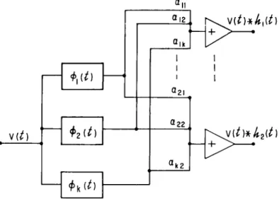
v(t - s) = 2 am(t,)<f>m(s), (0 < s < T). (5)
m = l
The </>m(s) are the coordinate axes of the M dimensional space and the am(t) are the coordinate magnitudes. An explicit identification of the axes need not be given at this time. They could, for example, be asso
ciated with the sampled data representation of v(t) in the time interval considered. The am would then be the amplitude samples obtained at equally spaced time increments ΔΤ and the <f>m the cardinal functions
sin
4 - -)
4 - =)
As will be seen, other representations are often more useful than the sampled data representation. The number of dimensions necessary to represent v(t) without error over the past T seconds is generally infinite. However, it is possible to use only the first M components if the data has bandwidth limitations or if one is willing to tolerate the errors associated with an approximation to the continuous data. The power spectrum or autocorrelation function of v(t) determines how large M should be for a given approximation error. These matters are discussed by Steiglitz (1966). He has some explicit results relating the number of samples to the approximation error in sampled data representations of signals that are not band limited. Such representations are employed when digital computer data processing is employed. Although Steiglitz's results are approximate in themselves, they can be used to estimate the sampling rate to be employed for the neural data obtained from the microelectrode. If this sample rate is R samples per second and T
seconds of data are to be considered at any one time, the dimensionality of the data is RT + 1. When analogue filtering techniques are em
ployed, they are themselves based upon sampling ideas, as in the case of the delay line or transversal filter, or their design specifications are obtained from the data by spectral analyses t h a t have used band limiting sampling techniques. Thus, the concept of a limit to the dimen
sionality of even non-bandlimited signals is an acceptable and accurate one.
The use of a multidimensional space permits a simple visualization of the problem associated with signal detection and identification. The vector representing the last T seconds of data will describe a trajectory in this space as time progresses. Because of their differing structures, noise and signals of various waveforms will tend to occupy different regions of the data space and to have different trajectories within it.
Separation of J different signals from noise and from one another is then possible by partitioning the space into J + 1 regions such t h a t when a data vector is found to lie in the J t h region of the space at a particular time, it is said to have been produced by the j t h signal source;
if it is in the Oth region, it is said to be noise. The partitioning of the space is a difficult task which must utilize a priori knowledge about the structure of the noise and signals encountered in order to yield optimum performance results. Since in many situations a priori knowledge about signal structure is not fully available, one of the functions of the data analysis procedures is to make signal structures more fully known for subsequent, more powerful investigations. For this reason, probably the most useful approach in the future to the problems of separation and analysis of neuronal signals will be in terms of adaptive pattern recog
nition procedures.
The establishment of data space partitions is done according to decision rules t h a t are generally of the maximum likelihood type. These insure some aspect of optimality to the decision process according to the particular criteria adopted. However, there is generally no partition which can yield perfect performance—a certain amount of error is inherent in the decision process and must be tolerated. Furthermore, as the complexity of the neural records increases with the number of units in a record, the performance level of even optimum systems deteriorates resulting in an upper limit to the complexity of the neural data records which can be profitably analysed. Carefully obtained single-unit records can be processed with negligible errors. When there are two units pre
sent, their occasional overlapping in time and their fluctuations in amplitude and shape give rise to unavoidable errors of identification.
When three or more neural units are recorded from, the situation
deteriorates further. It is not possible to set a limit to the number of units that can be handled simultaneously because this depends upon at least three factors: the resolvability of the particular units recorded from, the type of analysis which is to be performed on the data and the degree of confidence which is to be attached to the results. With these considerations in mind, we can proceed with discussion of the separation process.
F. Decision Procedures in Detection and Identification
The simplest separation problem is that of separating a known pulse shape from background noise. If the shape of the pulse is s(t) and it occurs in background of stationary, white noise, it is well known, see Davenport and Root (1958) for example, that the ratio of peak signal to r.m.s. noise is a maximum at the output of a filter, called a matched filter, whose impulse response h(t) is given by
h(t) = s(-t). (6) Decisions as to whether the filter output is produced by signal and noise
or noise alone can be made in an optimum fashion using only the am
plitude of the unidimensional vector representing the present output of the filter. The actual decision rule employed depends upon the a priori probability of occurrence of the signal, Ps, and the choice of costs asso
ciated with the decision errors of false alarm and false dismissal. In the simplest of situations s(t) occurs with a given strength or not at all. The decision rules is to decide that signal is present if the filter output ex
ceeds a threshold level determined by Ps and the cost function. If the threshold is not exceeded, noise only is said to be present. A thorough treatment of decision theory as applied to signal detection problems is given by Middleton (1961) and by Helstrom (1960).
The output of the matched filter is determined by the history of the nput to the filter over the past T seconds, the duration of the filter impulse response. If the input data can be represented by a finite number of samples obtained at the rate of R per second, the filter out
put can be considered as a weighted sum of the last RT + 1 samples rather than as a weighting applied to the continuously observed data over the same T seconds. That is, the integral representing the filter output can be replaced by an approximating summation
RT
x(t) = 2 h(m&T)v(t - mAT) [R = (ΔΤ)"1]. (7)
m = 0
The summation approximation is of great value when the data is to be
processed by digital computer. The output of the sampled matched filter is a projection of an RT + 1 dimensional data vector along the direction in data space determined by the signal vector itself. The decision as to signal presence or absence is made at the epoch of the signal, the time when in the absence of noise the filter output would be maximum. At the signal epoch the noise-free data vector has the same direction cosines as the time-reversed filter vector. Let us illustrate the idealized signal in Pig. 3(a) as only a two-dimensional vector. The com
ponents are s ^ ) and s(t2) where t2 — t± = ts. The input data v(t) is monitored continuously so t h a t v(t) and v(t — ts) are continuously available. As time proceeds, the vector representing these two quan
tities describes a trajectory as shown in Fig. 3(b). Noise is assumed absent. The epoch occurs when the trajectory intersects the radial line whose direction cosines are t h a t of the signal vector. (For simplicity this is assumed to occur only once per signal waveform.) In a noisy situation the trajectory will be perturbed and will tend to lie in a region around the trajectory as shown in Fig. 3(c). The size of this region is determined by the power and structure of the noise. The epoch of a noisy signal unless known a priori must be estimated and some error is inevitable. One reasonable estimation procedure is to call the epoch the time at which the output of the matched filter is at a maximum. Such a procedure is easy to instrument with a time derivative taker followed by a detector of negative going zero crossings. This sequence of opera
tions at the output of the matched filter generates a pulse at the time the filter output reaches its maximum value. The error involved in this estimation process will increase as the background noise power in
creases. Since the output of the matched filter is symmetric about the true epoch, the estimated epoch is unbiased with respect to the true epoch. I t is also a minimum variance and maximum likelihood estimate under the assumed conditions of stationary, normal white noise and a signal of known shape.
Another possible method for epoch estimation involves the estimation of the direction cosines of the received data vector in the ET + 1 dimensional sample space. The epoch is said to occur when the direction of the received vector approaches most closely to the direction of the noise-free signal. Thus epoch estimation would be done according to the equation
sin dvs(t) = min. (8)
The instrumentation required for this epoch estimation process appears to be more complex than t h a t for the previous estimate. The method is mentioned here only to illustrate t h a t alternative methods for epoch
(a)
\i(t-t$)
F I G . 3(a). An idealized signal (spike) waveform. A two-dimensional represen
tation is obtained by representing the waveform by its amplitudes at t1 and t2. (b) The trajectory of the signal vector in signal space when there is no noise present. The epoch occurs when the vector amplitude is a maximum, (c) The trajectory of the signal space when background noise is present. The dashed lines indicate the region in which the perturbed trajectory usually lies.
estimation exist. Under certain circumstances they may be the methods of choice.
Once the epoch has been estimated, the problem of single-signal detection is solved, for the only thing t h a t was to have been learned about the signal in this situation was its time of occurrence. If there are several different signals expected, each of known waveform, the prob
lem becomes to decide which, if any, has occurred. The solution to this problem is a straightforward generalization of the previous one. I t is to employ a matched filter for each of the waveforms and to decide the presence of t h a t waveform whose corresponding matched filter output is largest at each estimated epoch. This is true provided t h a t the im
pulse responses of the different filters are normalized with respect to their energies, i.e.
hi2(t) dt = constant (for all i).
Pig. 4 illustrates a matched filter system for the separation of three
k(t)\
M) I ut) 1
1
I
—> Thres hold L Gate 1
% 5
-> ^ _ *
1
%
1 Neg J ^ X i n g
| Det.
1 Neg J ^ X i n g
1 Pet.
I Neg J Z X m g
1 Det.
>
* <
>
Peak Ampl.
and Epoch
Sei.
F I G . 4. A m a t c h e d filter s y s t e m for d e t e r m i n i n g w h i c h of t h r e e w a v e f o r m s is p r e s e n t . T h e s y s t e m decision is b a s e d u p o n w h i c h of t h e filters h a s t h e g r e a t e s t o u t p u t w h e n t h e epoch occurs.
known waveforms in noise. A threshold detector in each filter channel is employed to discriminate against the identification of noise as a signal.
In this multiple-signal separation problem, the received data vector is projected by the matched filters onto the vectors of the sought-for sig
nals. The block diagrams indicate only the operations on the data, not how they are to be performed.
4*
If the solutions described for the separation of known signals in noise are optimum according to the decision criterion employed, t h a t of maximum likelihood, then all other solutions are inferior from this standpoint. However, the degree of inferiority of a given solution must be determined in any useful system performance evaluation, for it often occurs t h a t a non-optimum solution to a problem performs adequately and is capable of being implemented more easily and econo
mically t h a n the optimum one. Another consideration of equal, if not greater importance is whether the solution is capable of on-line opera
tion—separating signals as they occur in time with little or negligible delay between the receipt of a signal and its identification.
When the waveforms to be separated are unknown or partially known a priori, the matched filter approach is unsatisfactory since one cannot specify exactly the matched filters to be employed. This is the prevailing situation in experiments utilizing extracellular electrodes. Waveform separation can be accomplished but only after the structure of the wave
forms encountered have been determined. The separation process involves four steps:
(1) detection of the presence of spike activity,
(2) estimation of the shapes of the various spike waveforms,
(3) establishment of decision criteria based upon the differences of these shapes,
(4) testing of each waveform to determine the group it belongs to.
I n simple situations spikes produced by different neurons will be significantly different in amplitude so t h a t the first two steps can be taken quickly and easily, usually in the space of a few minutes or less in on-line operation. The amplitude ranges of the spikes from each of the several neurons are first determined and amplitude windows then employed to permit the on-line separation of the spikes. The process is similar when the data is recorded on tape and played back after the experiment. Here, however, the data occuring in the initial few minutes prior to the completion of the waveform analysis can be salvaged during replay by employing the decision rules used for the later portion of the run. Spike separation by amplitude discrimination is satisfactory when a record contains two or perhaps three units whose spike amplitude distributions are different enough from one another and from the noise as to overlap only slightly, if at all. Generally this implies t h a t the individual unit discharges are large in amplitude and stable, a situation indicating close proximity of the units to a nearly motionless recording electrode. The spike amplitude perturbations produced by the noise are not large enough to smear one spike amplitude distribution into another.
V(t) Data Filter (Fixed)
Threshold Detector
Gate
Waveform Estimates A Priori
Waveform Information
(o)
Waveform Classifier
and Epoch Est.
\ Decision Criteria
Coded - O Outputs for
f Waveform
" V Identity and Epoch
Data Filter (Variable)
*
Threshold Detector
Gate
Waveform Classifier Epoch Est and
Optimum Filter Computer and
Decision Rule Computer
; }
Coded Outputs for Waveform Identity and Epoch
(b)
F I G . 5(a). A rudimentary block diagram of a non-adaptive signal analyser.
The configuration of the system is fixed by a priori selection of the data filters and the criteria built into the waveform classifier, (b). A rudimentary block diagram of an adaptive signal analyser. The parameters of the data filter, the threshold detector and the waveform classifier are modified according to automatic analysis of the output data from the system. The system tries to optimize its performance in any given signal and noise situations.
Such a fortuitous combination of circumstances occurs infrequently.
Situations in which there is significant overlap in the amplitude dis
tributions of the spikes from different units are far more prevalent and data analysis procedures must be able to cope with them if multiunit studies are to be fruitful. Success in separating neural pulses is closely related to the kinds of subsequent analyses of interunit interactions.
Their sensitivity to the various errors of classification will differ and the effects of these errors on the hypothesis testing of unit interaction need to be determined. The sensitivity to decision errors undoubtedly increases with the number of units involved.
On-line performance of the processing system makes it necessary t h a t steps (1) through (4) above be completed in a single pass of the data with a minimum amount of time being devoted to the first three steps.
The simplest procedure is to perform the tasks in sequence, the outcome of each step providing the data to be used on the next. A more efficient and rapid way is to employ information feedback and use the waveform estimates of the fourth step to improve both the waveform estimation process of the second step and the setting of the decision boundaries of the third step. This so-called adaptive or learning procedure, see Nilsson (1965), possesses the further advantage t h a t it can be employed throughout the experiment to update waveform estimates as the data accumulates. Rudimentary block diagrams of a non-adaptive and an adaptive waveform separation system are shown in Fig. 5.
G. Orthogonal Representations of Neural Signals in the Data Space Regardless of whether one employs a non-adaptive or adaptive pro
cedure to separate waveforms, there must be some type of data filter upon whose output the decision-making process can be performed.
When there are several known waveforms, the data filter can be a set of parallel matched filters, one for each waveform. A possible extension of this to the situation where the waveforms are initially unknown is to use the spike data to synthesize adaptive filters matched to the indivi
dual waveforms. This idea has been pursued by at least one investi
gator, Smith (1963, 1964). However, when more than two or three waveforms are present, such a system can become quite cumbersome.
1. Orthogonal basis filters
There is a filter technique which follows the matched filter approach but avoids the need for a filter for each waveform. The technique involves approximate synthesis of the matched filters by means of a limited set of orthogonal filters whose impulse responses can be specified
SEPARATION OF NEURONAL ACTIVITY BY WAVEFORM ANALYSIS 9 9
beforehand and built into the system. If this set of filters—the basis filters—is chosen with care, it is possible to synthesize with an accept
ably small error the desired matched filter responses from linear com
binations of the selected filter functions. Acceptably small error here is taken to be one guaranteeing that the additional decision errors intro
duced by the use of the approximated matched filters are small.
Let the neural pulse waveforms to be separated be s^t), s2(t), s3(t), etc. They are members of an ensemble of neural spike waveforms. The matched filter impulse responses for each of these waveforms is given by
A,(i) = «,(-*)· (9) Let the basis filters employed be the first M members of the complete
set of orthonormal filters <j>k(t), where
JJ MW*(0 di = hik (i, k = 0, 1, 2, . . .). (10) The interval of time T for which the filters are defined is made at least as great as the duration of the longest spike waveform which can be encountered. If the complete set of filter functions is employed, it is possible to represent any h^t) without error by
00
h,(t) = Σ ««A(0 (o < t < T). (ii)
fc=0
For simplicity, the background noise is assumed to be white. When this is not so, the situation is somewhat more complex, but little is gained considering it here. For details see Middleton (1961). When only the first K filters of the basis set are employed, there is an error in approxi
mating hi(t) given by
ΛΓ Γ K
Jo L k=o (t) at. (12)
The integrated square error has been used for simplicity. An average error E(eK) over the set of all impulse responses associated with the spike waveforms can be defined as
E(eK) = jHP(h)eK(h)dh. (13)
The H space of possible filter functions h corresponds in one-to- one fashion with the S space of receivable neural spikes. p(h) is the
probability density of h in this space. With the idea of an average approximation error in mind, several questions can be posed:
(a) can we find a set of orthogonal filter functions whose first K members minimize E(eK)1
(b) can K be kept reasonably small and still yield an error which is consistent with acceptable spike separation performance?
(c) is the process which determines the optimum filters one which can be mechanized for on-line analysis of experimental data?
An interesting approach to the solution of these problems is that first employed by Huggins (1957). This involves the arbitrary a priori selection of the set of orthogonal filters to be employed. Typical choices for orthonormal filter responses are the Laguerre functions, the Hermite functions and sets of filters whose responses are determined by the Gram-Schmidt orthogonaHzation process. Aside from the problems of synthesizing these filters, difficulty is encountered in obtaining a reasonably close approximation to the waveforms of interest with a small number of the filter components. Selection of the set of basis functions to employ in a particular situation depends mostly on intui
tion with no explicit use of a criterion for goodness of fit. Nonetheless, such procedures have met with a certain amount of success.
2. Principal component determination of the basic functions
A somewhat different approach can be taken by employing the methods of principal component analysis which have had their origin in multivariate statistics. See Anderson (1958), Seal (1964) and Huggins (1960). John et al. (1964) and Donchin (1966) have employed these methods in the study of average evoked slow wave responses. The applicability of such methods to single-unit separation procedures seems to be great.
Consider a neural spike S(t) to be represented by its waveform samples at M instants of time equally spaced ΔΤ seconds apart. The spike is an M dimensional vector s whose coordinates are the sampled amplitudes {£(£m)}. Let this spike be one realization, originating from a particular neuron, of a neural waveform arising from a population of neurons, each generating its own "signature" waveform. The set of waveforms can be characterized by an a priori probability distribution in signal space. It is convenient, though not essential, to assume a normal distribution for the signal vectors. It is also appropriate to ignore the background noise in which the waveforms are observed, at least in so far as describing principal components is concerned. The back
ground noise becomes significant in considering procedures for estimat-
SEPARATION OF NEURONAL ACTIVITY BY WAVEFORM ANALYSIS 101
ing the principal components of a particular set of waveforms observed in noise.
The covariance matrix, Σ, of the neural waveforms is given for the sample amplitudes describing these waveforms by
Σ = E(S - μ)(5 - μ)' (14) where μ = E(S) is the mean signal for the population. The prime
symbol indicates the transpose operation.
The sample amplitudes can be considered to be the amplitudes of an orthogonal decomposition of the waveforms in terms of the cardinal functions. An orthogonal transformation can be applied to this sym
metric covariance matrix Σ yielding
λ = ψ Σ ψ (15) where ψ is an M x M orthogonal matrix. The total covariance of the
new matrix is the same as that of the old while all the off diagonal terms have been made to vanish. The new covariance matrix belongs to a set of orthogonal coordinates obtained by a rotation of the original coordinate axes. The coordinate vectors xVi are the eigenvectors of the transformation and are the columns of the matrix. The signal in the new coordinate representation is A, the vector of principle components of S.
Ä = VS. (16) The autocovariance of the jth component Ai9 is thus Ck. If we order the
eigenvectors according to the magnitudes of their eigenvalues, the auto
co variances, we obtain by definition the principal components of the original set of M dimensional random vectors. The first principal com
ponent contributes the greatest amount of covariance to the covariance matrix, the second has the next greatest contribution, and so on for the remaining principal components. The total number of principal com
ponents is, of course, equal to the number of dimensions of the random variables considered. The usefulness of the principal components lies in the ability of the first several of them to approximate the received waveforms with little error. The reason for this lies in the ordering of the components according to their co variances. We wish to use only the first K components whose combined covariance represents some given large fraction of the total covariance of all M components. Then the neural waveforms received can be represented by weighted sums of these K components with an approximation error which is only slightly larger than the approximation error incurred when all M of the original components are employed. Hopefully, K will be of the order of 5 or less.
The approximation error is most conveniently represented as of the integrated square type. The mean integrated square error over the class of waveforms received is just the sum of the covariances of the ignored principal components and is, by assumption, small compared with the energy in the retained components. Note that if the waveform being approximated is an estimated waveform, the principal compo
nents can provide no better an estimate of the true waveform than the original estimate. It is also important to note that the computation of the principal components is weighted according to the magnitudes of the waveforms received and the relative frequency with which they occur. Thus, a strong, frequently occurring spike will tend to lead to a set of principal components that is best suited to its features and not to the shapes of the smaller, less frequently occurring spikes. A more satisfactory set of principal components might be obtained by first normalizing the waveforms, or equivalently working with the correla
tion matrix (see Seal, 1964). This approach will not be dealt with here.
The magnitudes or weights of the individual principal components comprising the approximating sum are determined from the original (now noisy) data by the relationships
M
a, = 2 <Ay(<mMU 0' = 1,2,..., A'). (17)
m = l
The weights can be thought of in terms of equations (7) and (9) as the outputs of linear filters whose impulse responses are the time-reversed principal components φ}-( — t) and whose inputs are the data v(t):
M
aj(t) = 2 φ Δ Τ ) ^ ( - < + mAT) (mAT7 = tm). (18)
m = l
At time t = 0, the filter output is
M
ay(0) = £ φ Δ Γ ) ^ Α Γ ) . (19)
m = l
From this it can be seen that the estimates of the weights of the prin
cipal components of the data can be obtained from suitably designed linear filters, provided one knows the principal components and the signal epoch.
The discussion above has ignored the mean vector of the neural wave
form distribution. The reason for this is that it is convenient to assume that the mean is zero, that is, that initially positive waveforms are as likely to occur as initially negative. If there is reason to believe that the expected waveform is non-zero, then it would be of importance to
SEPARATION OF NEURONAL ACTIVITY BY WAVEFORM ANALYSIS 1 0 3
utilize this waveform information in estimating the epoch of the re
ceived waveforms. The mean waveform is the waveform of interest for a matched filter detector and is necessary in estimating the co- variance matrix of the received waveforms. It can be seen from this that assuming the expected neural waveform is zero leads to some simpli
fications in a principal component decomposition of the waveforms but contradicts the approach used in detecting waveform epochs. The difficulty is not as serious as it appears for satisfactory epoch detectors can be synthesized from the principal component filters resulting from the assumption of a zero expected signal.
The representation of the waveforms as vectors in a principal co
ordinate signal space leads to a relatively simple likelihood function for use in maximizing the detectability of the waveform. The equation for the log of the likelihood ratio L(t) under the situation where the signal coordinates are independent and normally distributed N(b, c) and exist in a background of white, normal noise is (Glaser, I960*),
L(t) = L0 + - ^ σ 2 ( σ.2 + Cj) (20)
Gj2 is the noise variance at the output of a filter whose impulse response is h(t) = ifjj(-t). The constant L0 is a function of σ2, cj and the a priori probability of a signal. According to this equation, the epoch for a waveform occurs when L(t) reaches a maximum. The optimum estimates for the principal component weights associated with the received waveform S(t) are obtained at this time and are given (Glaser,
1960),
+
(21)The previous paragraph describes the method for epoch estimation when the principal components are known. Initially, this is not the case and the epoch must be determined without such a priori signal information. If we assume that no waveform information whatever is available (except that the waveforms are less than T seconds in dura
tion), epoch detection is performed optimally according to the equation for the log of the likelihood ratio given by
L(t) = L 0 + \ l V A (22)
^ 3 = 1 σ
This is the epoch estimation rule to be employed in the initial acquisition
A more accessible reference is Van Trees (1968), Chapter 2-
of waveform data used for determining the principal components of the waveform. L0 = log (p/q) where p is the a priori probability of a wave
form occurring in time T and q = 1 — p.
The process of detecting the presence of initially unknown (more or less) waveforms and classifying them according to their waveform can now be specified:
1. The waveforms are unknown a priori except for being distributed normally N(b, c) in signal space with both b and c known. The wave
forms are imbedded in white background noise which is normal iV(0, σ2).
The epoch of a waveform is estimated according to equation (22) and M samples of its amplitude at equally spaced time points about the epoch are obtained. These amplitudes are stored in computer memory. N waveforms are detected and processed in this way. Of these, n1 will be of waveform Sl9 n2 of waveforms S2, and so on for all waveforms present.
There will also be n0 noise waveforms.
2. After receipt of the Nth waveform the estimated mean wave
form μ will be computed by the relation
μ ω = 4 ί » . ω (m=l,2,...,M) (23)
^ V i = 1
and the estimated covariance matrix for the waveforms by
± = ±li(Vi-{i)(Vi-iLy. (24)
The transformation to maximum likelihood estimates of the principal coordinates is carried out according to the process described in Sec.
11.3 et seq. of Anderson (1958). These estimates of the principal com
ponents are denoted by $m(i).
3. The filter impulse responses for the first K principal components are synthesized according to
Kit) = & ( - * ) (k= 1,2,...,K). (25) If a sampled data representation is employed,
h(t) = 4 ( - U ( m = 1 , 2 , . . . , i f ) . (26) 4. With the set of principal components determined, epoch estima
tion of the neuronal spikes is performed by computing L(t) according to equation (20) and determining when it reaches a maximum. The prin
cipal components are then read out and processed to yield the set of estimates as given by equation (21). These estimates are stored along with the estimated epoch. The next waveform detected is compared
SEPARATION OF NEURONAL ACTIVITY BY WAVEFORM ANALYSIS 1 0 5
with the first by measuring the distance between the waveform esti
mates in the K dimensional space,
£?
2= I (% - s
j2f. (27)
k = l
If the distance is less than some Dmin = cons x Κσ2, the waveforms are said to be identical and to have been produced by the same neuron.
σ2 is the sum of the noise powers in each of the K dimensions of the space.* It is obtained by measuring the noise-only output of the electrode when no units are present. If the distance between the wave
forms estimates is greater than Dmin, waveform 2 is considered to have been detected. The next waveform occurring is then estimated and com
pared with each of the two preceding waveforms to determine whether it is generated by neuron 1 or 2 or perhaps by a third neuron. If found to be generated by neuron 1, say, its waveform estimate is averaged with those of the earlier waveforms arising from neuron 1. As more spikes arising from neuron 1 are detected they are averaged with the preceding spikes to refine the waveform estimate for neuron 1. This is done for all waveforms in the record and permits account to be taken of slight changes occurring in the waveforms of the spikes as time progresses.
The decision boundaries that are established on the basis of the noise level in the record are thus made to follow the changes in the waveform shapes.
An alternative method of setting up decision boundaries when only two principal components are used can be briefly described. This me
thod, though as yet untested, seems to offer some promise. It presents the waveform data from the individual spikes as points on an oscillo
scope display generated by the computer. As the waveform data is received, the display will show build-up clusters of points corresponding to the different waveforms in the record (assuming the two components are capable of providing adequate resolution of the waveforms). Dis
plays such as this have been generated and photographed on conven
tional oscilloscopes by Glaser and Marks (1968). Fig. 6 illustrates one such display obtained from the optic nerve of limulus during several minutes of observation. Six different clusters are visible in the display.
Waveforms whose coordinates do not yield points falling within these
* This is true when Cj » σ>2, i.e., when the variance of the a priori distribution of waveforms is much greater than the noise output of the corresponding principal com
ponent filter. More generally, the variance of the estimated component magnitude is Cj afKcj + a2). Note also that the principal components are obtained from the original components by rotation so that the noise power outputs of the principal components filters are equal to those of the original orthonormal filters. With white noise a2 = σ2κ.