CAPOS: The bulge Cluster APOgee Survey I. Overview and initial ASPCAP results

June 2, 2021

CAPOS: The bulge Cluster APOgee Survey I. Overview and initial ASPCAP results

Doug Geisler^1,2,3, Sandro Villanova¹, Julia E. O’Connell¹, Roger E. Cohen⁴, Christian Moni Bidin⁵, José G.

Fernández-Trincado⁶, Cesar Muñoz^1,2,3, Dante Minniti^7,8,9, Manuela Zoccali^7,10, Alvaro Rojas-Arriagada^7,10, Rodrigo Contreras Ramos^7,10, Márcio Catelan^7,10,11, Francesco Mauro⁵, Cristían Cortés^7,12, C. E. Ferreira Lopes¹³,

Anke Arentsen¹⁴, Else Starkenburg^15,16, Nicolas F. Martin^14,17, Baitian Tang¹⁸, Celeste Parisi^19,20, Javier Alonso-García^21,7, Felipe Gran^10,7,22, Katia Cunha^23,24, Verne Smith²⁵, Steven R. Majewski²⁶, Henrik Jönsson²⁷, D.

A. García-Hernández^28,29, Danny Horta³⁰, Szabolcs Mészáros^31,32, Lorenzo Monaco⁸, Antonela Monachesi^2,3, Ricardo R. Muñoz³³, Joel Brownstein³⁴, Timothy C. Beers³⁵, Richard R. Lane⁶, Beatriz Barbuy³⁶, Jennifer Sobeck³⁷,

Lady Henao¹, Danilo González-Díaz^5,38, Raúl E. Miranda⁵, Yared Reinarz⁵, Tatiana A. Santander⁵

1 Departamento de Astronomía, Casilla 160-C, Universidad de Concepción, Concepción, Chile

2 Instituto de Investigación Multidisciplinario en Ciencia y Tecnología, Universidad de La Serena. Avenida Raúl Bitrán S/N, La Serena, Chile

3 Departamento de Astronomía, Facultad de Ciencias, Universidad de La Serena. Av. Juan Cisternas 1200, La Serena, Chile

4 Space Telescope Science Institute, 3700 San Martin Drive, Baltimore, MD 21218, USA

5 Instituto de Astronomía, Universidad Católica del Norte, Av. Angamos 0610, Antofagasta, Chile

6 Instituto de Astronomía y Ciencias Planetarias, Universidad de Atacama, Copayapu 485, Copiapó, Chile

7 Millennium Institute of Astrophysics, Santiago, Chile

8 Departamento de Ciencias Fisicas, Facultad de Ciencias Exactas, Universidad Andres Bello, Fernandez Concha 700, Las Condes, Santiago, Chile

9 Vatican Observatory, V00120 Vatican City State, Italy

10 Instituto de Astrofísica, Pontificia Universidad Católica de Chile, Av. Vicuña Mackenna 4860, 7820436 Macul, Santiago, Chile

11 Centro de Astro-Ingeniería, Pontificia Universidad Católica de Chile, Av. Vicuña Mackenna 4860, 7820436 Macul, Santiago, Chile

12 Departamento de Física, Facultad de Ciencias Básicas, Universidad Metropolitana de la Educación, Av. José Pedro Alessandri 774,7760197, Nuñoa, Santiago, Chile

13 National Institute For Space Research (INPE/MCTI), Av. dos Astronautas, 1758 – São José dos Campos – SP, 12227-010, Brazil

14 Université de Strasbourg, CNRS, Observatoire astronomique de Strasbourg, UMR 7550, F-67000 Strasbourg, France

15 Leibniz-Institut für Astrophysik Potsdam (AIP), An der Sternwarte 16, D-14482 Potsdam, Germany

16 Kapteyn Astronomical Institute, University of Groningen, Landleven 12, 9747 AD Groningen, The Netherlands

17 Max-Planck-Institut für Astronomie, Königstuhl 17, D-69117 Heidelberg, Germany

18 School of Physics and Astronomy, Sun Yat-sen University, Zhuhai 519082, People’s Republic of China

19 Observatorio Astronómico, Universidad Nacional de Córdoba, Laprida 854, X5000BGR, Córdoba, Argentina

20 Instituto de Astronomía Teórica y Experimental (CONICET-UNC), Laprida 854, X5000BGR, Córdoba, Argentina

21 Centro de Astronomía (CITEVA), Universidad de Antofagasta, Av. Angamos 601, Antofagasta, Chile

22 ESO Vitacura, Alonso de Córdova 3107, Santiago, Chile

23 Steward Observatory, The University of Arizona, 933 North Cherry Avenue, Tucson, AZ 85721-0065, USA

24 Observatório Nacional, Rua General José Cristino, 77, 20921-400 São Cristóvão, Rio de Janeiro, RJ, Brazil

25 National Optical Astronomy Observatory, 950 North Cherry Avenue, Tucson, AZ 85719, USA

26 Department of Astronomy, University of Virginia, Charlottesville, VA, 22904, USA

27 Materials Science and Applied Mathematics, Malmö University, SE-205 06 Malmö, Sweden

28 Instituto de Astrofísica de Canarias (IAC), E-38205 La Laguna, Tenerife, Spain

29 Universidad de La Laguna (ULL), Departamento de Astrofísica, 38206 La Laguna, Tenerife, Spain

30 Astrophysics Research Institute, Liverpool John Moores University, 146 Brownlow Hill, Liverpool L3 5RF, UK

31 ELTE Eötvös Loránd University, Gothard Astrophysical Observatory, 9700 Szombathely, Szent Imre H. st. 112, Hungary

32 MTA-ELTE Exoplanet Research Group

33 Departamento de Astronomía, Universidad de Chile, Camino del Observatorio 1515, Las Condes, Santiago, Chile

34 Department of Physics and Astronomy, University of Utah, 115 S. 1400 E., Salt Lake City, UT 84112, USA

35 Department of Physics and JINA Center for the Evolution of the Elements, University of Notre Dame, Notre Dame, IN 46556, USA

36 Universidade de São Paulo, IAG, Rua do Matão 1226, Cidade Universitária, São Paulo 05508-900, Brazil

37 Department of Astronomy, University of Washington, Seattle, WA, 98195, USA

38 Instituto de Física, Universidad de Antioquia, Calle 70 52-21, Medellín, Colombia June 2, 2021

ABSTRACT

arXiv:2106.00024v1 [astro-ph.GA] 31 May 2021

Context.Bulge globular clusters (BGCs) are exceptional tracers of the formation and chemodynamical evolution of this oldest Galactic component. However, until now, observational difficulties have prevented us from taking full advantage of these powerful Galactic archeological tools.

Aims.CAPOS, the bulge Cluster APOgee Survey, addresses this key topic by observing a large number of BGCs, most of which have only been poorly studied previously. Even their most basic parameters, such as metallicity, [α/Fe], and radial velocity, are generally very uncertain. We aim to obtain accurate mean values for these parameters, as well as abundances for a number of other elements, and explore multiple populations. In this first paper, we describe the CAPOS project and present initial results for seven BGCs.

Methods.CAPOS uses the APOGEE-2S spectrograph observing in the H band to penetrate obscuring dust toward the bulge. For this initial paper, we use abundances derived from ASPCAP, the APOGEE pipeline.

Results.We derive mean [Fe/H] values of -0.85±0.04 (Terzan 2), -1.40±0.05 (Terzan 4), -1.20±0.10 (HP 1), -1.40±0.07 (Terzan 9), -1.07±0.09 (Djorg 2), -1.06±0.06 (NGC 6540), and -1.11±0.04 (NGC 6642) from three to ten stars per cluster. We determine mean abundances for eleven other elements plus the mean [α/Fe] and radial velocity. CAPOS clusters significantly increase the sample of well-studied Main Bulge globular clusters (GCs) and also extend them to lower metallicity. We reinforce the finding that Main Bulge and Main Disk GCs, formed in situ, have [Si/Fe] abundances slightly higher than their accreted counterparts at the same metallicity.

We investigate multiple populations and find our clusters generally follow the light-element (anti)correlation trends of previous studies of GCs of similar metallicity. We finally explore the abundances of the iron-peak elements Mn and Ni and compare their trends with field populations.

Conclusions.CAPOS is proving to be an unprecedented resource for greatly improving our knowledge of the formation and evolution of BGCs and the bulge itself.

Key words. Stars: abundances; Galaxy: bulge; globular clusters: general

1. Introduction

A major goal of modern astronomy is to obtain an understanding of galaxy formation. An ideal tool for this would be a witness that was both present at the long-since-vanished epoch when most galaxies formed and yet still survives today to tell us its story.

We would also like many such witnesses, to corroborate their stories, that are readily observable and yield such critical information as composition, kinematics, and age in a well-understood, easily measured, accurate and precise way. Enter the globular clusters (GCs). They fulfill all of these attributes admirably and are among our most powerful cosmological archeology probes.

Globular clusters have proven to be especially vital in piecing together the mass assembly history of our own Galaxy, in particular the halo. The combination ofGaiaastrometry with the above astrophysical data for GCs has recently added a new dimension to our ability to trace back the story of how the Galaxy formed. Armed with the information provided by their integrals of motion, together with age and metallicity, we can now classify GCs as in situ or accreted, and even distinguish several major accretion events (e.g., Massari et al. 2019;Bajkova & Bobylev 2020;Kruijssen et al. 2020). The age-metallicity relationships of the GCs identified with the different proposed progenitors are tight and distinct, indicating that they were indeed likely independent entities that experienced unique chemical evolution histories (Kruijssen et al. 2019;Massari et al. 2019;Myeong et al. 2019). Additional clues from detailed abundances of key elements can further constrain our understanding of their particular chemical evolution histories (Horta et al.

2020).

However, such powerful studies require as complete a sample with as detailed knowledge as possible; without this, our ability to distinguish crucial complexities is compromised. This is graphically illustrated by comparing our vast knowledge of halo GCs (and thus the halo and its formation) with our very limited knowledge of their bulge and disk counterparts (and their respective Galactic components). We now believe most halo GCs were accreted, while the bulge and disk GCs were formed in situ (Barbuy et al. 2018;

Massari et al. 2019). The relative ease with which halo GCs can be, and have long been, observed compared to their bulge and disk counterparts means we have learned a tremendous amount about halo formation from them; unfortunately, this is not the case for the disk, or, especially, bulge GCs because of the observational difficulties detailed below. Thus, we face the embarrassing situation that we now know more about the accreted structures than our own homegrown GCs and the story of the main proto-Galaxy’s growth they trace.

The Galactic bulge (GB) is a fundamental part of our Galaxy. It is one of the most massive Milky Way components and is directly linked to the formation of various other Galactic structures, such as the bar and inner disk. Because galaxies formed from the inside-out, the metal-poor population in the inner few kiloparsecs (kpc) of the GB is the best place to search for the oldest Galactic stars (Tumlinson 2010;Carollo et al. 2016;Fragkoudi et al. 2020;Horta et al. 2021). Indeed, the rapid chemical evolution in the deep potential well of the GB means that even relatively metal-rich stars could be very old, potentially older than their even more metal-poor halo cousins, which were born and raised in much less massive satellites (Cescutti et al. 2008, Savino et al. 2020).

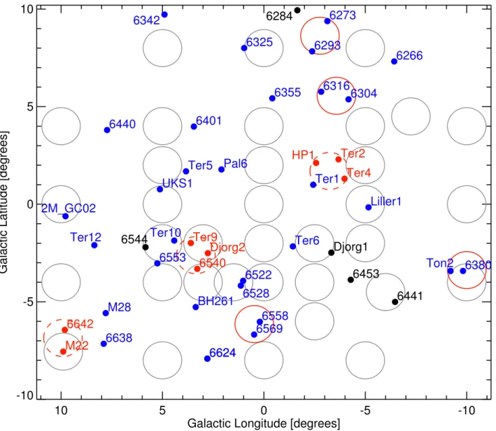
Bulge GCs (BGCs) are particularly important – as Shapley famously realized, the GB contains a disproportionately large number of them (43 in the central ±10^◦ × ±10^◦ area - Figure1) (Harris 1996, 2010 edition; hereafter H10). We now know that the GB possesses a GC system, independent from that of the halo (Minniti 1995b), that was formed generally in situ (Tissera et al. 2017;

Massari et al. 2019). Given our ability to derive absolute GC ages accurate to the∼ 0.5 Gyr level (e.g.,Saracino et al. 2016), depending on the method employed (seeCatelan 2018, for a recent review), the BGCs very likely include the oldest object in the Galaxy for which we can obtain an accurate age (Dias et al. 2016;Barbuy et al. 2018;Kerber et al. 2019). This will allow us (once we identify and measure it) to strongly constrain such profound questions as how long after the Big Bang the Galaxy began to form and how.

Unfortunately, until recently we had not been able to unleash the full power of the BGCs to help unravel the history of the GB.

Despite its proximity and central role as a primary primordial portion of the Galaxy, the GB has resisted detailed investigation due to the high foreground extinction that strongly limits optical observations. An additional complicating factor is crowding, which

10 5 0 -5 -10 Galactic Longitude [degrees]

-10 -5 0 5 10

Galactic Latitude [degrees] 6380

6440

6441 6522 6453

6528 6540

6544

6553

6569 6624

6624 6638

6642

Ter5 Ter4

Ter9 Ter6

HP1

Liller1

Djorg1 6401

2M_GC02

BH261

M22

M28 6558

Ter1 Ter2

Ter10 Ter12

Ton2 Pal6

Djorg2 UKS1

6266 6273

6293

6316 6304 6325

6355 6342 6284

Fig. 1.Central±10^◦× ±10^◦around the Galactic center. BGCs (i.e., withRGC ≤3.5kpc) are identified (generally with their NGC number) in blue and red, while other GCs withRGC >3.5 kpc are labeled in black. Gray circles show the locations of the SDSS-IV APOGEE-2S survey fields, while CAPOS fields are shown in red, with the dashed circles illustrating the CAPOS fields presented here. All CAPOS clusters are BGCs except for M22, which was observed simultaneously with the BGC NGC 6642. A final CAPOS BGC, NGC 6717, is offthe plot at (12.9^◦,−10.9^◦).

prohibits accurate measurements of individual stars. Field contamination is also highly problematic as what we see as the GB in projection is really the superposition of not only the bulge, but also the bar, the foreground (and background) thin (and thick) disk(s) and the halo. Furthermore, BGCs are generally buried in densely populated fields whose stars are difficult to distinguish photometrically from those of the BGC we want to study. Consequently, the two most comprehensive Hubble Space Telescope (HST)surveys of GCs - theAdvanced Camera for Surveys (ACS)survey (Sarajedini et al. 2007) and the HST UV Legacy Survey (Piotto et al. 2015) - were focused on halo and disk objects, almost totally avoiding those in the bulge.

However, the first two problematic effects are minimized by observing in the near-IR with high spatial resolution detectors, which have, fortunately, recently come on line. Moreover, contamination is now greatly alleviated via Gaia astrometry (Gaia Collaboration et al. 2016,2018). Also, high-precision radial velocities such as those provided by theApache Point Observatory Galactic Evolution Experiment (APOGEE)(Majewski et al. 2017) bring an additional powerful membership discriminant. The combination of all these recent advances finally enables us to effectively exploit the extraordinary Galactic archeology attributes of BGCs.

Recognizing the importance of near-IR observations of the GB, the Vista Variables in the Via Lactea (VVV) survey (Minniti et al. 2010) was granted a 5 year ESO Public Survey on the ESO 4m VISTA telescope to map the GB (and adjacent disk) inYZ JHK_s with the aim of studying its structure and a vast variety of fascinating objects hidden there, with BGCs as one of the top priorities.

The VVV has proven to be extremely successful, so much so that a 3 year extension, dubbed the VVV eXtended survey, or VVVX for short, is now underway (Minniti 2018). The VVVX extends the spatial coverage of near-IR imaging of the bulge out to 10^◦in both Galactic latitude and longitude - the entire area of Fig.1.

The VVV team has taken full advantage of this unique database to study BGCs. They have discovered many new GC candidates (e.g.,Moni Bidin et al. 2011;Minniti et al. 2011,2017a,b;Palma et al. 2019), found dual horizontal branches in two metal-rich GCs (Mauro et al. 2012), investigated structural parameters (Cohen et al. 2014), studied variable stars (e.g.,Alonso-García et al. 2015),

and provided the deepest VVV-based color-magnitude diagrams (CMDs) to date (Cohen et al. 2017). In addition, and of particular importance, follow-up very deep near-IR HST (Cohen et al. 2018) and Gemini-S GeMS (e.g.,Saracino et al. 2016) images have been obtained for many BGCs. GeMS is a multiconjugate adaptive optics instrument that produces very high spatial resolution images in the near-IR, with image quality competitive with HST but on an 8m telescope. The superb image quality of both HST and GeMS in the near-IR makes BGCs accessible, for the first time, to the deep photometry required to derive accurate ages. The VVV images, as pioneering as they are, are simply too shallow and the spatial resolution is woefully inadequate for this purpose.

For example, the depth of the exquisite GeMS NGC 6624 data (Saracino et al. 2016), reaching>4 mag below the main sequence turn-off(MSTO) inKsand>3 mag fainter than VVV, reveals faint features previously only theoretically predicted, such as the main sequence (MS) knee - the blueward inflection in the curvature of the lower MS - allowing age measurements with 0.5 Gyr precision from purely near-IR ground-based imaging, even in the cluster center. Similar deep GeMS and HST optical-near-IR images for a number of BGCs are now in hand, providing an unprecedented photometric database for a large number of BGCs.

However, to measure the best age, and hence pin down the earliest formation epoch of the Galaxy with the smallest error, requires both deep high spatial resolution photometry and high spectral resolution spectroscopy to derive the detailed abundances required for isochrone fitting. The main factors that are still sorely lacking are good [Fe/H], [α/Fe], and [CNO/Fe] values for BGCs, all of which are very scarce. All CMD-based age diagnostics are very sensitive to these key elements. Given our exquisite near- IR photometry exemplified by NGC 6624 (also see, e.g., HP1 - Kerber et al.(2019), NGC 6256 - Cadelano et al.(2020)), the single remaining dominant uncertainty on BGC ages is their abundances. Incredibly, most of these invaluable objects have only poor estimates of the overall metallicity - based on a variety of techniques, making a very heterogeneous sample - and little to no abundance information beyond this.

Fortunately, with the arrival of the APOGEE southern instrument APOGEE-2S, filling in the missing link of abundances in BGCs is now feasible. APOGEE is a high-resolution, near-IR spectroscopic survey, which is part of the fourth iteration of the Sloan Digital Sky Survey (SDSS-IV;Blanton et al. 2017). APOGEE-2S, a copy of the original APOGEE instrument built for the Sloan telescope in the north for SDSS-III, is attached to the du Pont 2.5m telescope at Las Campanas Observatory in Chile, opening access to the Southern Hemisphere and the GB as part of SDSS-IV.

Given their importance, the SDSS-IV survey has targeted some BGCs with APOGEE-2S. Nevertheless, this is an enormous global Galactic and even extragalactic survey, covering hundreds of thousands of stars, and simply cannot afford to study a single part of the Galaxy in complete detail. SDSS-IV is surveying 35 fields within the central 10^◦×10^◦ GB area on the sky. These fields include a number of GCs. However, the GB is more than just an area on the sky: It is a distinct Galactic component with a well-known spatial distribution, and not all of the objects found in this area are actually inside the GB - some are in the foreground or background. Taking 3.5 kpc as a limiting Galactocentric radius for the GB (Schultheis et al. 2017;Massari et al. 2019), the H10 catalog of GC properties includes 55 BGCs. We note thatBica et al.(2016) use both the spatial distribution, with a 3 kpc cutoff, as well as metallicity to arrive at a final list of 43 BGCs. For the present, we only concern ourselves with the three-dimensional spatial location, using a 3.5 kpc limit, and ignore metallicity, orbit, and origin when refering to BGCs. Of the 43 GCs lying in the central 10^◦×10^◦(which includes most but not all BGCs), 6 lie well beyond this Galactocentric radius, including 4 of the SDSS-IV GCs, leaving a total of 37 bona fide BGCs. SDSS will only observe a handful of these. Initial small-scale studies of APOGEE results based on SDSS-III and -IV observations are given inSchiavon et al. (2017),Tang et al.(2017), andFernández-Trincado et al.

(2019). Indeed,Mészáros et al.(2020) present the APOGEE sample of 44 clusters, of which only 8 are bona fide BGCs according toMassari et al.(2019). Of these, they dismiss all but 2 as either not having a large enough sample of well-observed members or having too high reddening. This represents less than 4% of the total number of BGCs known, a disconcertingly low value. If one is searching for the oldest GC in the Galaxy, and aiming to take full advantage of the wealth of astrophysical detail these key objects can provide by performing a definitive study of the BGC system, as complete a sample as possible is essential.

Hence the CAPOS project, the bulge Cluster APOgee Survey (the b is silent). The primary goal of CAPOS is to obtain detailed abundances and kinematics for as complete a sample as possible of bona fide members in true BGCs, using the unique advantages of APOGEE to complement the much smaller sample observed by SDSS-IV, via Chilean access to APOGEE-2S through the CNTAC (the Chilean National Telescope Allocation Committee). We aim to help gather the first definitive database on the BGC system, search for the oldest object in the Galaxy with an accurate age, study the very complex nature of the GB and uncover any underlying correlations, determine BGC velocities and orbits and investigate multiple populations in the BGC system, and compare them to their halo (and disk) counterparts. As noted above, this demands as complete a sample as possible. The power of this approach is to establish the population of BGCs as an ensemble, finally placing them on a level with and in the context of their hither-to much better-studied halo counterparts, and thus fill in our picture of all Milky Way GC systems, especially the in situ BGCs.

CAPOS originally targetted 20 cataloged BGCs, with the goal of bringing the number of bona fide BGCs observed by APOGEE to 28, over half of the total, with CAPOS supplying almost three-fourths of the observed sample. CAPOS will, together with the SDSS-IV data, provide a legacy database of the BGC system. This will provide much better and completely self-consistent spectroscopic metallicities than currently available for all the observed BGCs, as well as derive detailed abundances for some 20 elements with a wide variety of nucleosynthetic origins, precise to∼0.05 dex. Current knowledge of their abundances is limited to only a few, if any, spectra of individual stars, and/or crude photometric metallicity estimates, or even integrated light measurements in many cases. We will also obtain excellent radial velocities. Many of the BGCs have only limited or even nonexistent velocity information.

CAPOS also targets any recently discovered BGC candidates that can be observed serendipitously with cataloged BGCs, given the large field of view of APOGEE. These include such intriguing objects as FSR1758, a newly discovered massive BGC that is the eponymous member of the Sequoia dwarf galaxy (Barbá et al. 2019;Massari et al. 2019;Myeong et al. 2019;Villanova et al. 2019;

Romero-Colmenares et al. 2021), as well as any other candidates from the VVV survey (e.g.,Palma et al. 2019).

We will also search for multiple populations (MP) in BGCs. The study of MP in GCs has revolutionized our understanding of their formation and evolution but so far has been limited almost exclusively to non-GB, non-metal-rich GCs. CAPOS will open up

the regime of high metallicity to detailed MP studies, since BGCs include the highest metallicity of all Milky Way GCs. APOGEE includes lines of the light elements C, N, O, Na, Mg, Al, and Si, which are essential to tracing MP.

We aim to observe 5-10 members per cluster to derive accurate mean abundances, search for and characterize MP, and constrain scenarios for the formation of MP.

Given the compact size of BGCs and fiber collision limitations, most fibers will be available for objects outside of the GCs. To optimize the science return, CAPOS targets hundreds of GB field giants per plate. Abundances for Fe andα-elements and velocities will delineate the kinematics and chemistry of distinct GB components. Our fields also overlap K2 mission areas (Howell et al.

2014), and we will exploit K2 data to explore Galactic archaeology using asteroseismology (Johnson & APOKASC Collaboration 2016). Gaia astrometry, K2 asteroseismology, CAPOS stellar parameters, and VVV photometry allow us to trace the GB chemical evolution, resolved into its different components.

Finally, we also target metal-poor candidates from theExtremely Metal-poor BuLge stars with AAOmega survey (EMBLA) (Howes et al. 2016) andPristine Inner Galaxy Survey (PIGS)surveys (Starkenburg et al. 2017a;Arentsen et al. 2020). The metal- poor tail of the bulge/inner Galaxy has not yet been studied in detail since the number of metal-poor stars is extremely small compared to the more metal-rich stars that dominate in the inner Galaxy. In APOGEE DR16, there are only∼50 stars with [M/H]

< −2.0 located within (|l,b|) < 10^◦ (Ahumada et al. 2020). Past and current high-resolution surveys targeting metal-poor stars only contain a handful with−2.5 <[Fe/H]<−1.5 (Howes et al. 2016;Duong et al. 2019;Lucey et al. 2019). Larger samples of metal-poor inner Galaxy stars are needed to disentangle this complicated area of the Galaxy, where multiple Galactic components overlap. Additionally, the contribution of disrupted GCs to the metal-poor inner Galaxy is currently poorly constrained. It is crucial to obtain high-resolution follow-up spectra for metal-poor inner Galaxy stars, providing detailed chemical abundances combined with kinematics, which can help to disentangle different stellar populations. Finally, it is also of great interest to search for the most metal-poor stars in the inner Galaxy, which are likely to be among the oldest in the Milky Way (e.g.,Tumlinson 2010;Starkenburg et al. 2017b;Horta et al. 2021).

The CAPOS/PIGS collaboration aims to greatly increase the number of (very) metal-poor inner Galaxy stars with high-resolution spectroscopy available. The Pristine survey (Starkenburg et al. 2017b) is a photometric survey that employs metallicity-sensitive CaHK photometry from MegaCam on the CFHT to efficiently search for the most metal-poor stars in the Galaxy. Its main focus is on the Galactic halo and dwarf galaxies; additionally, there is a sub-survey toward the GB (PIGS). There are two CAPOS fields with PIGS targets. Based on the results from the first field, we expect to increase the number of [M/H]<−2.0 stars within (|l,b|)<10^◦ by 60% compared to APOGEE DR16, and we expect to increase the number of stars with [M/H]< −1.5 by 30%. Most of these stars will also have low/intermediate resolution optical/calcium triplet spectra available from the PIGS follow-up efforts (Arentsen et al. 2020).

In this first CAPOS paper, we include an overview of the project and initial results based on theAPOGEE Stellar Parameters and Chemical Abundance Pipeline - ASPCAP (García Pérez et al. 2016) analysis of all BGC CAPOS data released in DR16 (Ahumada et al. 2020). As can be seen in Fig.1, the other H10 BGCs CAPOS observed include: NGC 6273, NGC 6293, NGC 6304, NGC 6316, NGC 6380, Ton 2, NGC 6558, NGC 6569, and NGC 6717 (this final BGC is outside Fig.1). The paper is organized as follows: We first present details of the selection of clusters as well as targets within clusters. We also discuss how field stars were selected, including bulge field stars, K2 stars, and stars from the EMBLA and PIGS surveys. Next, the observations and reductions are discussed. We then present a number of key results from the ASPCAP analysis, starting with the final determination of cluster members based on a variety of criteria. We discuss the ASPCAP atmospheric parameters and their errors. Next we derive the mean metallicity, [α/Fe], and heliocentric radial velocity of each cluster, and compare these values to the literature. We then investigate mean abundances for a number of other well-determined elements. Multiple populations in the clusters are then investigated, followed by the results for Fe-peak elements. Finally, we summarize our main conclusions.

2. Sample selection 2.1. Cluster selection

The initial CAPOS goal was to observeallBGCs that appear in the H10 catalog and lie within the central 10^◦×10^◦ area of the bulge that were not planned to be observed with APOGEE-2S as part of the SDSS-IV survey. This would have provided a complete sample of H10 BGCs within this central bulge area, and would have included, together with the SDSS clusters, some 70% of the cataloged BGCs. However, this proved to be too ambitious, given the time constraints imposed by the limitations on the instrument, Chilean access, and the extensive Covid-19 LCO shutdown coming in the last year of APOGEE-2. In the end, we were able to observe a total of 16 CAPOS BGCs. This, combined with the SDSS clusters, will bring the total to 24 of 55 BGCs, a nearly majority sample that doubles the total covered by APOGEE over those observed by SDSS alone. In addition, we will observe a few BGCs or candidates that are not in the H10 catalog that lie within the same APOGEE field as cataloged targets.

Specific APOGEE fields to observe were selected via several criteria. First, given the limited time granted, we prioritized fields that included multiple BGCs within the same large APOGEE field of view, which is over 1^◦in radius. We also prioritized the most metal-poor BGCs, given our goal of searching for the oldest of these. Everything else being equal, the least-studied clusters were deemed especially interesting. Fields that included new GC candidates (Minniti et al. 2017a,b;Barbá et al. 2019;Palma et al. 2019) were also prioritized. Finally, due to the hour angle restrictions of APOGEE, especially during the highly competitive bulge season, we emphasized fields at the extreme RA ends of the bulge. The initial three fields observed and reported on here include two with three BGCs each and a third with a BGC and a non-BGC. This last field is at the extreme eastern end of the central bulge field, and includes NGC 6656 (M22). Although M22 is outside of our limiting Galactocentric radius for BGCs, it is an interesting GC in its own right, having been the subject of considerable debate as to whether or not it has an intrinsic metallicity spread (e.g.,Norris &

Freeman 1983;Mucciarelli et al. 2015), and is readily observed simultaneously with the BGC NGC 6642. M22 will be the subject

Table 1.Basic positional data for all CAPOS clusters.

Cluster ID α(J2000.0) δ(J2000) L(^◦) B(^◦) APOGEE

hh:mm:ss ^◦: ⁰: ⁰⁰ Field

NGC 6273 17 02 37.8 -26 16 04.7 356.87 9.38 357+09-C NGC 6293 17 10 10.2 -26 34 55.5 357.62 7.83 357+09-C NGC 6304 17 14 32.3 -29 27 43.3 355.83 5.38 356+06-C NGC 6316 17 16 37.3 -28 08 24.4 357.18 5.76 356+06-C Terzan 2 17 27 33.1 −30 48 08.4 356.32 2.30 357+02-C Terzan 4 17 30 39.0 −31 35 43.9 356.02 1.31 357+02-C HP1 17 31 05.2 −29 58 54 357.44 2.12 357+02-C NGC 6380 17 34 28.0 -39 04 09 350.18 -3.42 350-03-C Ton 2 17 36 10.5 -38 33 12 350.80 -3.42 350-03-C Terzan 9 18 01 38.8 −26 50 23 3.61 -1.99 003-03-C Djorg 2 18 01 49.1 −27 49 33 2.77 -2.50 003-03-C NGC 6540 18 06 08.6 −27 45 55 3.29 -3.31 003-03-C NGC 6558 18 10 17.6 -31 45 50.0 0.20 -6.02 000-06-C NGC 6569 18 13 38.8 -31 49 36.8 0.48 -6.68 000-06-C NGC 6642 18 31 54.1 −23 28 30.7 9.81 -6.44 010-07-C NGC 6656 18 36 23.9 −23 54 17.1 9.89 -7.55 010-07-C NGC 6717 18 55 06.0 -22 42 05.3 12.88 -10.90 013-11-C Note:Equatorial coordinates, L and B are from H10.

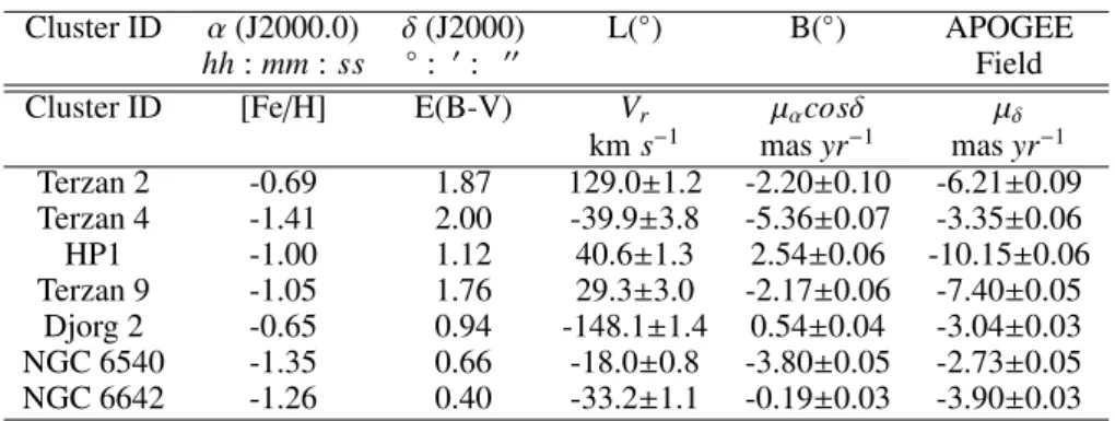
Table 2.Basic parameters from the literature for CAPOS I clusters.

Cluster ID α(J2000.0) δ(J2000) L(^◦) B(^◦) APOGEE

hh:mm:ss ^◦: ⁰: ⁰⁰ Field

Cluster ID [Fe/H] E(B-V) V_r µ_αcosδ µ_δ

kms⁻¹ masyr⁻¹ masyr⁻¹ Terzan 2 -0.69 1.87 129.0±1.2 -2.20±0.10 -6.21±0.09 Terzan 4 -1.41 2.00 -39.9±3.8 -5.36±0.07 -3.35±0.06

HP1 -1.00 1.12 40.6±1.3 2.54±0.06 -10.15±0.06

Terzan 9 -1.05 1.76 29.3±3.0 -2.17±0.06 -7.40±0.05

Djorg 2 -0.65 0.94 -148.1±1.4 0.54±0.04 -3.04±0.03

NGC 6540 -1.35 0.66 -18.0±0.8 -3.80±0.05 -2.73±0.05

NGC 6642 -1.26 0.40 -33.2±1.1 -0.19±0.03 -3.90±0.03

Note:[Fe/H] and E(B-V) are from H10.Vrand astrometry are fromBaumgardt et al.(2019).

of another paper in this series. Finally, the GC candidate Minni 51 (Minniti et al. 2017a) was observed along with 3 BGCs in one of our fields. We note that our CAPOS observations find no convincing evidence for the reality of Minni 51, i.e. there is no clustering in metallicity:radial velocity space for the 9 targets, supporting the null finding byGran et al.(2019), and we will not discuss this object further here.

We note that all of the targets designated BGC here are also classified as bona fide BGCs byBica et al.(2016), based on their spatial distribution and metallicity, and as Main Bulge objects byMassari et al.(2019) as judged by their kinematics.Pérez-Villegas et al.(2020) also identify all of our clusters as bulge/bar from their orbits. The recent reassessment byBajkova & Bobylev(2020) maintains the same association as Massari for our objects except for NGC 6540, which they label a Disk GC. We will keep the Massari designations but note that CAPOS velocities will be used to reinvestigate in detail this association in a forthcoming paper.

For completeness sake, we report in Table 1 basic positional data for all CAPOS clusters, including the APOGEE field ID, while Table 2 lists additional basic parameters from the literature for the clusters we report on here. We note that our BGC sample covers a wide metallicity range, but not the very highest BGC metallicities, which reach nearly solar abundance, and that the reddenings are generally quite large.

2.2. Cluster target star selection

For each cluster, available spectroscopic, photometric, and astrometric information were all leveraged wherever possible to maxi- mize the number of bona fide cluster members that were observed, and exclude disk and bulge field star contaminants. Specifically, the following criteria were used to assign priorities, from highest to lowest:

– Stars with extant high-resolution spectroscopy, noting that only 5 of our 16 CAPOS clusters have published high-resolution spectroscopy, and only two in the current sample. This is to ensure membership and allow comparison with previous studies.

– Stars that are members based on radial velocity and metallicity information from low-resolution spectroscopy, typically using the CaII triplet. Such information was available for 10 of 16 CAPOS clusters, drawn primarily fromMauro et al.(2014),Dias et al.(2016), andGeisler et al.(2021).

– Stars that are likely members based on their proper motions (PMs) and uncertainties. For clusters observed in the first (2018) season (the current sample), ground-based PMs were employed where available, especially those derived from multi-epoch VVV photometry (Contreras Ramos et al. 2017), since Gaia data were not yet available. For the remainder of the clusters, a similar procedure was followed to select members from all candidates with valid PMs from Gaia DR2, typically applying a 2σclip to the two-dimensional proper motion errors of stars in the magnitude range of APOGEE targets (see below) to select candidate members.

– Near-IR PSF photometry from the VVV survey (Cohen et al. 2017;Alonso-García et al. 2018), matched to 2MASS, was used to reject foreground disk stars via a cut in (J−KS) color blueward of the cluster red giant branch

The last requirement on cluster targets is set by the available exposure time, which was a total on-source time of 5h or 6h per cluster initially. Following the strategy adopted for the APOGEE survey of GCs (Zasowski et al. 2017), targets were required to have 7.5<H<13 to ensure useful signal-to-noise. In practice, these cuts imply that all BGC members actually observed should be GK giants.

With a list of candidate members in hand for each cluster, targets were assigned to individual plates, assigning the brightest stars first within each priority itemized above to maximize the total number of candidates observed. By far the primary factor limiting the number of candidate members that could be observed in each cluster is the 56⁰⁰fiber collision limit for the southern APOGEE spectrograph, which is why careful prioritization of candidate members as described above is crucial to maximize the number of likely cluster stars assigned fibers. We employed multiple visits, changing out bright stars in different visits, to observe as many probable cluster members as possible (see Sect. 3). The number of visits was decreased as the survey progressed, but for the current sample, 6 visits were obtained for field 003-03-C and 5 each for fields 357+02-C and 010-07-C. Both GC and field targets are initially selected in three magnitude ranges: H ≤ 11, 11 ≤ H ≤ 12.2, and 12.2 < H ≤ 12.8, for single, 2-3 and> 3 visits, respectively, with the aim of achieving roughly similar S/N for the final added spectra.

2.3. Bulge field star selection

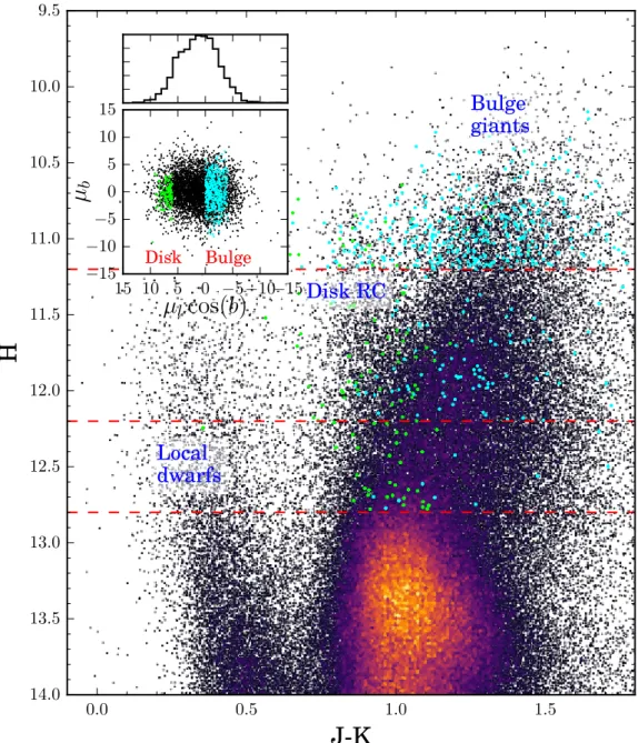
The APOGEE 2.1^◦ diameter circular FOV covers an area that is not only large enough to contain more than one GC in some favorable cases, but also allows us to design observations that complement GC targets with surrounding field populations. In this regard, a selection function was designed to also include bulge and disk field giants, in the fields observed within the initial CAPOS project, namely fields 010-07-C, 003-03-C, and 357+02-C. These fields were observed before the release of Gaia DR2, and thus necessitated a different procedure to include PM criteria than was the case for subsequent observations. The selection was designed to observe bulge RGB stars, plus a fraction of disk red clump (RC) stars. The selection was based on photometry and relative PMs computed from VVV psf photometry (Contreras Ramos et al. 2017). The selection function is illustrated in Fig.2. In this figure, the CMD of a typical bulge region is displayed (in this case, the 003-03-C field). The dominant bulge RC population is prominent around (J−K=1.1,H=13.5), from which the sequence of intrinsically brighter and redder RGB stars emerges. The bright vertical plume at J-K=0.4 corresponds to Solar Neighborhood dwarf stars, while the vertical, less prominent sequence, at J-K=0.8 - 0.9, is due to disk RC stars at progressively larger distances from the Sun.

Using VVV PMs, the vector point diagram (VPD) was constructed for the whole set of available stars in a few magnitude ranges/cohorts (see inset in Fig.2). From this diagram, two kinematical selections are performed to obtain clean samples from the bulge RGB and disk RC. This is done by selecting stars from the bulge and disk overdensities in the VPD, avoiding the overlap area in between them. Disk stars are selected as those with 6≤µ_lcos(b)≤10, while bulge stars are those with−4≤µ_lcos(b)≤0.

The resulting kinematically selected samples are highlighted in the VPD and the CMD displayed in Fig.2as green and cyan dots, respectively. For subsequent observations, we used the same procedure but supplemented with Gaia DR2 PMs.

2.4. K2 star selection

Kepler K2 targets were selected from the K2 Galactic Archaeology Program (K2GAP), described byStello et al.(2015,2017).

Specifically, the K2 sample is composed of red giants located in the K2 campaigns 7 and 11, which are overlapping with several surveys, including VVV, Gaia, and 2MASS. These stars present Hmagnitudes ranging from 7.2 to 12.1. The asteroseismology observations performed by K2 provide us with accurate measurements of stellar masses, ages, and radius for red giants (Kallinger et al. 2010). K2 targets appear in the initial CAPOS field 357+02-C, and were given high priority.

2.5. EMBLA star selection

The EMBLA survey contains some of the oldest and most metal-poor stars in the bulge and indeed in the Galaxy (Howes et al.

2016). Of course, some fraction of the EMBLA stars are metal-rich due to contamination. EMBLA sources overlap spatially with two initial CAPOS fields, 003-03-C and 010-07-C. EMBLA targets in these fields were selected and prioritized using a combination of preexisting information and observing constraints imposed by APOGEE-2S magnitude and fiber collision limits (Zasowski et al.

2017;Santana et al. 2021). In the selected fields, EMBLA sources were given relatively high priority and chosen at random at the fiber configuration stage.

0.0 0.5 1.0 1.5

J-K

9.5

10.0

10.5

11.0

11.5

12.0

12.5

13.0

13.5

14.0

H

Local dwarfs

Disk RC

Bulge giants

−15

−10

−5 0 5 10

15

µ

cos(b)

−15

−10

−5 0 5 10 15

µ

Disk Bulge

Fig. 2.Selection function of bulge and disk field giants.Main panel:Annotated CMD of a typical bulge field (003-03-C) is shown as a Hess diagram. The horizontal red dashed lines indicate the magnitude limits adopted to select cohorts, as described in the main text.Inset panel:

µlcos(b) vs.µbVVV PM diagram. The black points correspond to a random 2500 field star subsample with small errors in PMs. The cyan (green) points in both panels display the kinematically selected bulge (disk) giants from the magnitude ranges displayed in the main panel.

2.6. PIGS star selection

Metal-poor PIGS targets are selected using the metallicity-sensitive PristineCaHKphotometry. TheCaHK photometry, which is already cross-matched withGaiaDR2 (Gaia Collaboration et al. 2016,2018), is also cross-matched with 2MASS (Skrutskie et al.

2006). We select stars withH<12.8 and 2MASS quality f lagph_qual=AAA, to have stars in the CAPOS brightness regime with good quality 2MASS photometry. The Gaia and PristineCaHKphotometry are corrected for extinction using theGreen et al.(2018) reddening map. We limit the selection to a color range of 0.9<(BP−RP)0<1.5, where metal-poor giant stars are expected to lie.

A cut is added on the (parallax/parallax_error)<0.3, to remove contamination from foreground stars with significant parallaxes.

We finally sort the stars by the following metallicity-sensitive color: (CaHK−BP)0−2.5(BP−RP)0, and select the 100 stars with the smallest values, which are expected to be the most metal-poor. The next best 200 stars are provided as back-up targets. The efficiency of this type of selection has been presented inArentsen et al.(2020). The CAPOS/PIGS collaboration began with the 2019 observations, so no results are included in this work, which contains only earlier observations.

3. Observations and reductions

CAPOS time was granted via the CNTAC as an External Program to APOGEE (Majewski et al. 2017), part of SDSS-IV (Blanton et al. 2017). The APOGEE instruments are high-resolution, near-infrared H-band spectrographs (Wilson et al. 2019) observing from

both the Northern Hemisphere at Apache Point Observatory (APO) using the SDSS 2.5m telescope (Gunn et al. 2006), assisted by the NMSU 1m (Holtzman et al. 2010), and the Southern Hemisphere at Las Campanas Observatory using the 2.5m du Pont telescope (Bowen & Vaughan 1973). Stars are targeted using selections described inZasowski et al.(2013),Zasowski et al.(2017),Santana et al.(2021) andBeaton et al.(2021). Spectra are reduced as described inNidever et al.(2015) and analyzed using the APOGEE Stellar Parameters and Chemical Abundance Pipeline (ASPCAP,García Pérez et al. 2016), which compares the observed spectra with a complete spectral library of synthetic spectra (e.g.,Zamora et al. 2015) A detailed analysis of the accuracy and precision of the stellar parameters and abundances can be found inHoltzman et al.(2018) andJönsson et al.(2018). Our analysis uses results from the 16th Data Release (DR16) of the SDSS collaboration (Ahumada et al. 2020), which is the first data release containing data from the southern instrument. Further explanations and assessments of this data release can be found inJönsson et al.(2020).

CAPOS was awarded time over a number of different semesters. The assigned CAPOS nights were June 20-21 (CNTAC program CN2017B - 37) and July 21, 2018 (CN2018A - 20), June 14 and 19 (CN2018B - 46) and July 9-10, 2019 (CN2019A - 98), and May 30, June 27, and August 10, 2020 (CN2019B - 31), for a total of 10 nights. Unfortunately, all three 2020 nights were lost to LCO closure due to Covid-19, but an additional BGC was very recently observed after APOGEE-2S operations reinitiated in late October while the bulge was still observable. No further CAPOS observations will be possible as SDSS-IV has now ceased operations. DR16 only includes data taken by June 2019 and thus only includes three CAPOS fields. These three fields include seven BGCs, M22, and a candidate GC fromMinniti et al.(2017a). M22, along with other CAPOS clusters observed subsequently to June 2019, will be studied in subsequent papers.

CAPOS observations were carried out by the SDSS APOGEE-2S survey team in the same manner as for the survey observations (seeAhumada et al. 2020, for details), except that CNTAC time was granted as entire nights. Unfortunately, given the rather strict hour angle limits of APOGEE-2S, the bulge is only observable during about half the night, even during bulge season in the long winter nights. This of course severely limits the number of possible CAPOS observations, and caused us to descope the project by observing significantly fewer fields and less time per field than originally planned. Any unusable time during each assigned CAPOS night was returned to SDSS for normal survey operations.

To obtain as large a sample of cluster members as possible to map potential chemical inhomogeneities within a cluster, in particular multiple populations, our goal is to observe 5-10 members per cluster. However, given the small size of GB clusters and the fiber collision limit, we are able to put only a small number of fibers on probable cluster members for each pointing. To mitigate this problem, CAPOS generally observes each field with multiple visits (with the standard 1 hour exposure per visit). The number of multiple visits per cluster was originally set to six, but we trimmed this to five after the first run and eventually even lower, given the above time constraints. The number of targets observed in each cluster is maximized by replacing bright (H<11) stars with other bright stars after a single visit, (or after three visits for 11<H<12.2), while fainter (12.2<H<12.8) targets are observed for all visits to attain the required S/N (≥70 is the standard minimum for ASPCAP). Our stringent selection criteria, including Gaia DR2 astrometry for later observations, helped maximize the observation of actual members.

APOGEE-2S has 300 fibers per plate. Typically 250 fibers are placed on science targets, with the remaining 50 divided between 15 standard stars and 35 fibers allocated to sky. So apart from cluster targets, we are able to observe hundreds of field stars per pointing. We have no problem filling the remaining non-GC fibers with good targets. Results from these subsidiary projects will be presented in forthcoming papers.

As a Contributed CNTAC APOGEE data set, the CAPOS reductions and pipeline analysis were carried out in the standard way for APOGEE data. Details are presented inAhumada et al.(2020). In particular, the data are first processed by the APOGEE pipeline (Nidever et al. 2015), which yields heliocentric radial velocity. Then stellar parameters are determined using the ASPCAP pipeline (García Pérez et al. 2018) to derive abundances for some 20 chemical elements for stars withS/N > 70. Line lists are fromShetrone et al.(2015) andSmith et al.(2021). Each spectrum is analyzed independently in an automated manner. A detailed analysis of the accuracy and precision of these parameters and abundances is given inHoltzman et al.(2018) andJönsson et al.

(2018). Several improvements have been implemented for DR16, as delineated inAhumada et al.(2020) and further investigated inJönsson et al.(2020). ASPCAP is known to yield more precise abundances for stars with metallicities [Fe/H]>−1.7 (Leung &

Bovy 2019). All of the BGCs reported on here have H10 metallicities that well exceed this minimum.

4. ASPCAP results

Results presented here are based on the DR16 ASPCAP analysis. Future papers will explore different analysis techniques such as deriving our own atmospheric parameters and using BACCHUS (Brussels Automatic Code for Characterizing High accUracy Spectra - Masseron et al. 2016), which will allow us to compare CAPOS results in closer detail with those derived for BGCs observed by the SDSS APOGEE survey and analyzed using this code and independent atmospheric parameters (Masseron et al.

2019;Mészáros et al. 2020).

4.1. Cluster membership selection

APOGEE DR16 provides accurate radial velocities (RVs, accurate to typically∼0.05 km s⁻¹) and metallicites (accurate within∼0.10 dex) determined by ASPCAP. In addition, it includesGaiaDR2 astrometric data, which is available for essentially all our observed stars, although not available for target selection prior to the 2018 observations presented here. With accurate RVs and metallicities from APOGEE and PMs fromGaiain hand, CAPOS leveraged both surveys to optimally select bona fide cluster member stars from the original targets observed.

Each CAPOS field reported on here encompassed 2−4 cataloged plus candidate clusters in the designated FOV (see Fig. 1).

Targeted stars, including all bulge, K2, EMBLA, and PIGS filler targets observed by APOGEE, were extracted from the DR16 data

Table 3.CAPOS mean cluster metallicity, [α/Fe], radial velocity and proper motion for members.

Cluster ID [Fe/H]^a [α/Fe]^a Vra µ_αcosδ^b µ_δ^b Nfibers Nmembers N1G

(dex) (dex) (km s⁻¹) (masyr⁻¹) (masyr⁻¹)

Terzan 2 −0.85±0.04 0.26±0.01 133.2±1.4 −2.23±0.21 −6.36±0.16 58 4 2

Terzan 4 −1.40±0.05 0.21±0.01 −48.3±3.5 −5.08±0.26 −2.96±0.20 74 3 2

HP 1 −1.20±0.10 0.22±0.00 39.8±4.0 2.57±0.13 −10.15±0.10 43 10 2

Terzan 9 −1.40±0.07 0.16±0.05 68.1±4.3 −2.16±0.23 −7.39±0.19 55 9 4

Djorg 2 −1.07±0.09 0.27±0.04 −150.2±4.7 0.59±0.15 −3.17±0.14 73 7 4

NGC 6540 −1.06±0.06 0.26 −14.4±1.1 −3.89±0.14 −2.79±0.12 57 4 1

NGC 6642 −1.11±0.04 0.25 −56.1±1.1 −0.17±0.08 −3.98±0.06 51 3 1

aMean APOGEE [Fe/H], [α/Fe], radial velocities, and associated standard deviations for cluster members.

bMeanGaiaDR2 proper motions and associated errors for CAPOS cluster members.

Note:Only cluster members with spectra with S/N>70 are included to determine mean values.

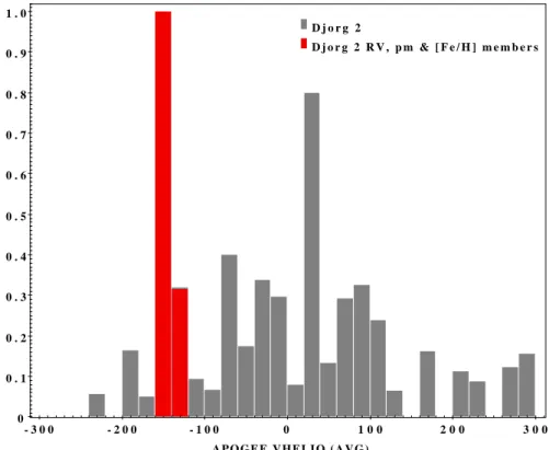
set by their designated APOGEE field name, then separated into individual cluster target lists. Cluster targets with S/N<70 were discarded, following previous similar studies (e.g.,Mészáros et al. 2020). Histograms of APOGEE RVs were constructed for each field, weighted by error, binned and normalized to show the relative number of stars per RV peak per field. An example is shown in Fig.3. This in fact is not a typical case - all other GCs showed single peaks. It should be noted that many CAPOS clusters have not been extensively studied, and some not at all, so the H10 catalog was consulted only as a guide. Target stars were then isolated within a 3σclip from the mean RV values found in the histograms. In the case of Djorg 2, which shows two peaks (Figure3), we treated both as possible cluster means until only one met our robust final criteria.

As a guide to identify each cluster’s location, density maps inGaiaPM space were created using the cluster’s central coordinates in a radius somewhat larger than the half light radius listed in H10. The potential RV cluster members were over-plotted onto the same PM space. A second subset of possible members was then isolated in the region identified as the cluster’s position in the PM density maps. The RV and PM candidate members were then cross matched to create yet another subset of cluster member candidates satisfying both criteria. To help ensure our candidate member stars arebona fidecluster members, we include an additional step using GaiaDR2 PMs by plotting their space motion projected onto the great circle coordinate system. Candidates that showed skewed directions from that of the bulk of other candidates were discarded, regardless of RV. An example is shown in Fig.4.

Finally, we use cluster metallicity as a membership criterion. Given the∼0.10 dex absolute uncertainty for ASPCAP metallici- ties, we consider any remaining member candidates as metallicity outliers if their ASPCAP [Fe/H] falls>3σfrom the cluster mean (see Table3). This final criterion resulted in very few candidate members being discarded, typically one per cluster.

Our method appears to be robust, though restrictive, and yields a high probability our final selections are indeed bona fide cluster members. Table3lists our final derived mean cluster parameters and associated standard deviations, including APOGEE ASPCAP metallicity, [α/Fe], and heliocentric RV, our derived mean cluster PM values based on Gaia, the number of allocated fibers, the number of final cluster members, and the number of 1G stars (see below). For comparison, Table 2 lists the mean PMs for CAPOS clusters fromBaumgardt et al.(2019) who, unfortunately, do not publish individual cluster member values. We find the mean cluster PMs between the two studies are in good agreement. We note that the percentage of allocated fibers on a cluster that turned out to correspond to cluster members ranged from 4% in Terzan 4 to 23% in HP1, with a average of 12%.

4.2. ASPCAP atmospheric parameters

As part of the pipeline, ASPCAP derives atmospheric parameters simultaneously from a global fit to the entire spectrum, and then detailed abundances for some 20 elements by fitting the spectral lines to models using these atmospheric parameters. We tested the reliability of the ASPCAP stellar parameters and abundances, first checking for any trend of iron abundance in each cluster as a function of the effective temperature. We indeed find a significant positive gradient of increasing metallicity with temperature of similar magnitude for most clusters.

A possible systematic effect on chemical abundances with effective temperature for previous ASPCAP data releases has been studied in the literature, both in GCs (Mészáros et al. 2013;Masseron et al. 2019), and field stars (e.g.,Zasowski et al. 2019). In particular, it is known (Jönsson et al. 2018) that ASPCAP overestimates (with respect to the optical studies taken as reference) effective temperatures as well as surface gravities for so-called second generation (2G) stars, i.e. stars with abundance patterns typical of stars believed to have been born from gas polluted by first generation (1G) stars to form a subsequent generation(s), leaving a present-day cluster displaying MP.

One of the best indicators of 1G versus 2G stars is their N abundance, as N is very substantially increased from 1G to 2G stars, by an amount that can approach or exceed 1 dex (see below). Of course, N is also increased by various dredge-up episodes ocurring on the RGB as a result of normal stellar evolution (Kraft 1994;Gratton et al. 2000). However, this does not affect the overall metallicity.

Fig.5shows that there is indeed a trend within each of our clusters for stars with the highest [N/Fe] abundances (2G stars - hereby defined as those with [N/Fe]>0.7) to also show a higher metallicity than their 1G counterparts (and that 2G stars generally have higherTeffthan their 1G counterparts). If ASPCAP overestimatesTefffor 2G stars, it will also overestimate [Fe/H] since higherTeff

generally means fainter spectral lines and a higher metallicity is required to fit a given line. Gravity does not have as great an impact on abundances asTeff, at least for giants. It is expected, given the ASPCAP methodology, that there will be systematic differences for other, possibly all, elements for 2G stars.

- 3 0 0 - 2 0 0 - 1 0 0 0 1 0 0 2 0 0 3 0 0 A P O G E E V H E L I O ( A V G )

0 0 . 1 0 . 2 0 . 3 0 . 4 0 . 5 0 . 6 0 . 7 0 . 8 0 . 9 1 . 0

D j o r g 2

D j o r g 2 R V , p m & [ F e / H ] m e m b e r s

Fig. 3.Histogram of ASPCAP heliocentric radial velocity for all stars in the area around the BGC Djorg 2. Our final Djorg 2 members are shown in red, while field stars that did not meet the radial velocity, proper motion, and/or metallicity selection are in gray.

-27.90 -27.88 -27.86 -27.84 -27.82 -27.80 -27.78

270.35 270.40

270.45 270.50

270.55

Dec (degrees)

RA (degrees) Djorg 2 RV members (~ -150 km s^-1) Djorg 2 RV and PM members

Fig. 4. Proper motion vectors on the sky for radial velocity members of Djorg 2. Red corresponds to stars selected as fi- nal cluster members from their common radial velocity, proper motion, and metallicity, while gray shows field stars. The black circle indicates a radial velocity and proper motion member that was discarded due to its discrepant metallicity.

For this reason, abundances for 2G stars are typically derived using independent atmospheric parameters, along with boutique software, such as BACCHUS, instead of relying on ASPCAP. We will use such a technique in a subsequent paper, but for the purposes of this study we decided to correct the metallicity of 2G stars as follows: We first derive the mean cluster [Fe/H] of all 1G stars. We then calculated the offset of each 2G star from its cluster mean and found a very consistent mean difference of+0.06±0.01 dex for all 2G stars. We then subtracted this value from the ASPCAP [Fe/H] of all 2G stars, and use this corrected [Fe/H] value to derive the mean metallicity and its error, which is the standard deviation convolved with an assessment of the error in this correction, which are given in Table3. We recognize that, although most stars are either low or high N (1G or 2G, respectively - see Figures 8 and 9), there are some intermediate stars and this is a simplification.

It is unfortunately very difficult to estimate the effects of this systematic error on the abundances of the other species for 2G stars because the intrinsic dispersion of light elements and the higher measurement errors of heavy elements will blur any underlying trend. For this initial paper, we will only use 2G stars in deriving the mean [Fe/H] (in combination with 1G stars) as described here, and to qualitatively investigate MP, and use only 1G stars to derive mean abundances for all other elements, as given in Tables3 ([α/Fe]) and4. The number of 1G stars is given in the last column of Table3.

Fig. 5.Difference in [Fe/H] as a function of [N/Fe], with the cluster mean for 1G stars ([N/Fe]<0.7) taken as the zero point: red=Terzan 2, magenta

=Djorg 2, cyan=HP1, yellow=NGC 6540, blue=Terzan 9, orange=Terzan 4, green=NGC 6642. Symbol size is directly proportional toT_eff. A clear trend is found for 2G (higher [N/Fe]) stars to have both a higherT_effand [Fe/H] than 1G stars in the same cluster.

4.3. ASPCAP abundances

A number of studies have investigated how well different atomic species are measured with APOGEE spectra, including comparisons of ASPCAP abundances with those from applications of boutique programs to APOGEE spectra as well as to other studies, e.g.

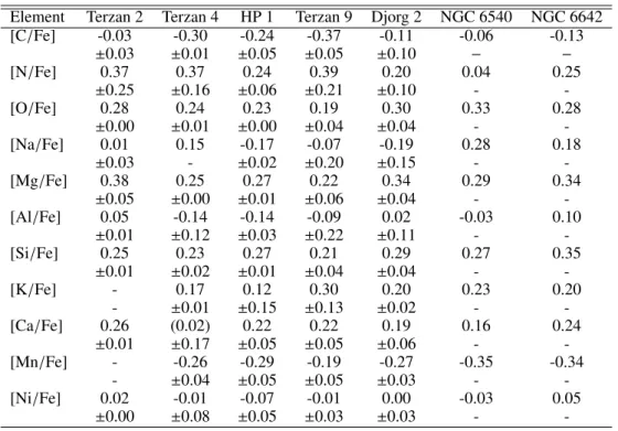
from optical spectra. Most recently,Jönsson et al.(2020) carry out this procedure for all stars in DR16, whileMasseron et al.(2019) andMészáros et al.(2020) restrict their studies to GCs in the north and south, respectively. The general consensus of these studies is that ASPCAP abundances for 1G stars with metallicity around -1 dex, as is the case for our current sample, are deemed to have well-determined values for at least the following elements: C, N, O, Na, Mg, Al, Si, K, Ca, Fe, Mn, and Ni, so we restrict our current study to these species.

C, N, O, Na, and Al are the key light elements to investigate MPs. Na is more problematic than the other elements listed in terms of precise measurement with ASPCAP. There are only two Na I lines, which are very weak, especially at the relatively low metallicities of our sample (although they are seen in the coolest stars in M107, with a metallicity of−1:Masseron et al.(2019), and located in a region heavily blended by telluric features. Nevertheless, we keep Na due to its important role in investigating MP, but emphasize that the results should be viewed with caution.Fernández-Trincado et al.(2020) investigate differences between ASPCAP and BACCHUS abundances for some 1000 presumed 1G field stars with -2<[Fe/H] < −0.65. They found ASPCAP

to overestimate the abundances of N, O, and Al by about 0.2 dex with a scatter of about 0.1 dex. Nevertheless, we will use the ASPCAP abundances at face value.

As for the α-elements, which traditionally include O, Mg, Si, S, Ca, and Ti, all are measured with ASPCAP. In addition, ASPCAP provides an overall estimate of a global (α-elements relative to metal abundance), denoted [α/M], essentially [α/Fe], in its fit to determine the atmospheric parameters, fitting all of theα-elements simultaneously while keeping their relative abundances identical. We consider O as an element strongly affected by MP (and indeed ASPCAP O abundances are particularly problematic for 2G stars -Masseron et al. 2019). Mg and Si can also be affected by MP, but to a lesser extent (e.g.,Bastian & Lardo 2018). We further note that both S and Ti are not well measured by APOGEE (Jönsson et al. 2020). So we are left with Mg, Si, and Ca as the best APOGEEαtracers. Happily, all three of these keyα-elements are very precisely measured in APOGEE.Nidever et al.(2020) investigate how ASPCAP abundances of these elements compare to the high-resolution optical studies ofCarretta et al.(2009) for 58 1G giants in 11 GCs with a wide range of metallicity, covering the range of our BGCs studied here. They found a mean offset of 0.17 dex for [Mg/Fe] with a standard deviation of 0.08 dex, an offset of 0.09 dex for [Si/Fe] with a standard deviation of 0.07 dex, and an offset of 0.16 dex for [Ca/Fe] with a standard deviation of 0.16 dex, with all of the offsets being in the same sense - with the ASPCAP values lower than the Caretta values.Fernández-Trincado et al. (2020) investigate Mg and Si abundances in their large field star sample and find small mean ASPCAP overestimates but null within the errors. Again, we will use the ASPCAP abundances at face value.

Nidever et al.(2020) also verified that the parameter-level [α/M] value yields abundance patterns consistent with those of the individualαelements but is more precise, and therefore seems the current best choice for the ASPCAP [α/Fe] abundance. There is currently some freedom to choose the best estimate of the overall [α/Fe] abundance in APOGEE, including the parameter-level [α/Fe] (e.g.,Nidever et al. 2020), [Mg/Fe] (e.g.,Rojas-Arriagada et al. 2019), [Si/Fe] (e.g.,Horta et al. 2020), or some combination thereof.

The fundamental element Fe is well measured in ASPCAP. We note that ASPCAP metallicities, at least for 1G stars in other GCs, are generally in good agreement with those of other high-resolution studies.Nidever et al.(2020) compare the metallicities of stars in 26 GCs with ASPCAP metallicities ranging from -0.6 to -2.3 with those of other high-resolution studies, and found a mean offset of 0.06 dex to higher metallicity for ASPCAP and a scatter of 0.09 dex, whileFernández-Trincado et al.(2020) find an offset of 0.11±0.11 dex in the opposite sense when comparing ASPCAP to BACCHUS abundances. We will simply use the ASPCAP values, after correcting the metallicities of 2G stars as described above. Our mean [Fe/H] values are given in Table3. Of the various Fe-peak elements measured by ASPCAP, including V, Cr, Mn, Co, Ni, and Cu, the most reliable are Mn and NiJönsson et al.(2020), so we include only these here.

We include K in our analysis but only give our mean values, saving details for this and other elements for a future paper. The mean abundances and their standard deviations from 1G stars are reported in Table4for the 11 elements we study besides Fe and α. We note that we exclude from cluster means the very rare cases where an element in a given star was flagged as being unreliable.

4.4. Fundamental cluster parameters: Mean metallicities, [α/Fe] abundances, and radial velocities

The mean metallicity, designated [Fe/H], of a GC is the primary parameter detailing its chemical composition. The next most salient composition indicator is the abundance of theαelements, designated as [α/Fe]. Finally, RVs provide crucial information regarding membership, internal kinematics and the cluster’s orbit. Despite the critical importance of these parameters, among the most fundamental for our understanding of a cluster’s formation and subsequent chemical and dynamical evolution, the current state of our knowledge of these parameters for BGCs is woefully inadequate. This is particularly true for most of our current sample.

Indeed, CAPOS was devised to address this problem for as many BGCs as possible, taking advantage of the powerful APOGEE instrument, which was designed to deliver high-precision RVs and abundances for a large number of elements, including Fe and all of the species consideredα-elements. In this section we discuss the ASPCAP results for [Fe/H], [α/Fe], and RV for our initial CAPOS clusters.

4.4.1. Metallicity

We first discuss Fe. Fe is generally synonymous with metallicity. The metallicity of a cluster has long been recognized as an excellent tracer of its nature, and gives invaluable insight into the cluster’s supernova enrichment history.Zinn(1985) first divided Galactic GCs into halo and disk systems primarily based on [Fe/H]. ThenMinniti(1995b) argued that some of the inner metal-rich GCs belong to the GB. More recently,Bica et al.(2016) used [Fe/H] to discriminate between BGCs and non-BGCs, with a division at -1.5. They noted that the metallicity distribution for BGCs show two peaks - the traditional one associated with BGCs at [Fe/H]=-0.5 but also another one around -1, which in fact is of equal if not greater strength. They point out that these lower metallicity clusters lie at the low end of the bulge field-star metallicity distribution and are the best candidates for the oldest Galactic objects. It turns out that all of our present CAPOS sample are members of the lower-metallicity subset. Unfortunately, the metallicity information for our clusters, and indeed most BGCs, comes from a hodgepodge of sources with a large range of precision and accuracy, but mostly of relatively poor reliability and not involving near-IR capabilities to overcome the extinction problem. Although all of our clusters have been investigated before, at least in terms of metallicity and radial velocity, the metallicity estimates are generally based on relatively low-quality indices, such as the slope or color of the RGB in a CMD or low-resolution optical spectra. Only two of the sample have been the subject of high-resolution spectroscopic studies, and only one of these within the last 15 years.

Needless to say, such studies are very inhomogeneous, and make it very difficult to compare abundances in one cluster derived with one method to that in another derived with a different method. CAPOS now provides unprecedented metallicities, of much higher