arXiv:2007.14261v1 [math-ph] 28 Jul 2020
ISOTROPY OF SPACE
JUDIT X. MADAR ´ASZ, MIKE STANNETT, AND GERGELY SZ´EKELY
Abstract. Given any Euclidean ordered field,Q, and any ‘reasonable’ group, G, of (1+3)-dimensional spacetime symmetries, we show how to construct a model MG of kinematics for which the set Wof worldview transformations between inertial observers satisfiesW =G. This holds in particular for all relevant subgroups ofGalcPoi, andcEucl(the groups of Galilean, Poincar´e and Euclidean transformations, respectively, wherec∈Qis a model-specific parameter corresponding to the speed of light in the case of Poincar´e transfor- mations).
In doing so, by an elementary geometrical proof, we demonstrate our main contribution: spatial isotropy is enough to entail that the setWof worldview transformations satisfies eitherW⊆Gal,W⊆cPoi, orW⊆ cEuclfor some c >0. So assuming spatial isotropy is enough to prove that there are only 3 possible cases: either the world is classical (the worldview transformations between inertial observers are Galilean transformations); the world is rela- tivistic (the worldview transformations are Poincar´e transformations); or the world is Euclidean (which gives a nonstandard kinematical interpretation to Euclidean geometry). This result considerably extends previous results in this field, which assume a priori the (strictly stronger) special principle of relativity, while also restricting the choice ofQ to the fieldRof reals.
As part of this work, we also prove the rather surprising result that, for any Gcontaining translations and rotations fixing the time-axist, the requirement thatGbe a subgroup of one of the groupsGal,cPoiorcEuclis logically equiva- lent to the somewhat simpler requirement that, for allg∈G:g[t] is a line, and ifg[t] =tthengis a trivial transformation (i.e.gis a linear transformation that preserves Euclidean length and fixes the time-axis setwise).
1. Introduction
Physical theories conventionally define coordinate systems and transformations using values and functions defined over the field of reals,R. However, this assump- tion is not well-founded in physical observation because all physical measurements yield only finite-accuracy values — even quantum electrodynamics (QED), one of the most precisely tested physical theories, is only accurate to around 12 decimal digits [OHDG06]. Since we have no empirical reason to make this assumption, it is worth investigating what happens to our expectations of physical theories if we generalize by assuming less about the physical quantities used in measurements. In this paper, we assume only that every positive element in the ordered field of quan- tities has a square root, but it is worth noting that special relativity can also be modelled over the field of rational numbers [MS13], in which even this assumption fails. It remains an open question whether the new results presented here generalize over arbitrary ordered fields.
2010Mathematics Subject Classification. Primary 51P05 (83A05, 70B99); 20A15; 46B20.
1
Starting in 1910, Ignatovsky’s [Ign10a, Ign10b, Ign11] attempt to derive special relativity assuming only Einstein’s principle of relativity initiated a new research direction investigating the consequences of assuming the principle of relativity with- out Einstein’s light postulate. However, Frank and Rothe [FR11] quickly identified (1911) that hidden assumptions were implicitly used by both Einstein and Igna- tovsky, and it is still not uncommon over a century later to find hidden assumptions in related works.
One notable investigation was that of Borisov [Bor78] (see also [Gut82, §10, pp. 60-61]). Borisov explicitly introduced all the assumptions used in his framework investigating the consequences of the principle of relativity. Then he showed that there are basically two possible cases: either the world is classical and the worldview transformations between inertial observers are Galilean; or the world is relativistic and the worldview transformations are Poincar´e transformations.1
In [MSS19], we made Borisov’s framework even more explicit using first-order logic, and investigated the role of his assumption that the structure of physical quantities is the field of real numbers. We showed that over non-Archimedean fields there is a third possibility: the worldview transformations can also be Euclidean isometries.2
In this paper, we present a general axiom system for kinematics using a simple language talking only about quantities, inertial observers (coordinate systems), and the worldview transformations between them. Our axiom system is based on just a few natural assumptions, e.g., instead of assuming that the structure of physical quantities is the field of real numbers we assume only that it is an ordered field Q in which all non-negative values have square roots. Using this framework, we investigate what happens if instead of the principle of relativity we make the weaker assumption that space is isotropic. We show that isotropy is already enough to ensure that the worldview transformations are either Euclidean isometries, or Galilean or Poincar´e transformations; see Theorem 5.5 (Classification).
The investigation presented in this paper is part of the Andr´eka–N´emeti school’s general project of logic-based axiomatic foundations of relativity theories, see e.g., [AMN06, AMN07, AMNS12, AN14]. Friend and Molinini [Fri15, FM15] discuss the significance of this project and the underlying methodology from the viewpoints of epistemology and explanation in science. One important feature of using a first- order logic-based axiomatic framework is that it helps avoid hidden assumptions, which is fundamental in foundational analyses of this nature. Another feature is that it opens up the possibility of machine verification of the results, see e.g., [SN14, GBT15].
2. Framework
We are concerned in this paper with two sorts of objects,(inertial) observers and quantities, which we represent as elements of non-empty sets IOb and Q, respectively.
Observers are interpreted to be labels for inertial coordinate systems. Quantities are used to specify coordinates, lengths and related quantities, and we assume that
1Metric geometries corresponding to these two structures also appear among Cayley-Klein geometries; see, e.g., [Str16] and [PSS17,§6].
2That the principle of relativity is consistent with world view transformations being Euclidean isometries has previously been shown by Gyula D´avid [D´av90].
Q is equipped with the usual binary operations,·(multiplication) and + (addition);
constants, 0 and 1 (additive and multiplicative identities); and a binary relation,≤ (ordering).
Although the results presented here can also be generalized to higher-dimensional spaces (though not necessarily lower-dimensional ones — see Sect. 8), we assume for definiteness that observers inhabit 4-dimensional spacetime, Q4, and locations in spacetime are accordingly represented as 4-tuples over Q. We often write~p,~q and~r to denote generic spacetime locations.
For each pair of observers k, h ∈ IOb, we assume the existence of a function wkh: Q4→ Q4, called the worldview transformation from the worldview of h to the worldview of k, which we interpret as representing the idea that observers may see (i.e. coordinatize) the same events, but at different spacetime locations:
whatever is seen byhat~p is seen byk atwkh(~p).3
Formally, this framework corresponds to using a two sorted first-order language where the models are of the following form
M= (IOb,Q,+,·,0,1,≤,w),
where: IOb and Q are two sorts; + and·are binary operations onQ; 0 and 1 are constants onQ;≤is a binary relation onQ; andwis a function fromIOb×IOb×Q4 to Q4. In this language, the worldview transformation between fixed observersk andhcan be introduced as:
wkh(t, x, y, z)def=w(k, h, t, x, y, z).
3. Axioms
In this section, we describe the general axiom system, KIN, used to represent kinematics in this paper. Additional axioms representing spatial isotropy and the special principle of relativity will be introduced in Section 4.
3.1. Quantities. We assume that (Q,+,·,0,1,≤) exhibits the most fundamen- tal algebraic properties expected of the real numbers (R), so that calculations can be performed and results compared with one another. We also assume that square-roots are defined for non-negative values (i.e. thatQ is aEuclidean field [EOM20]).
AxEField: (Q,+,·,0,1,≤) is a Euclidean field, i.e. a linearly ordered field in which every non-negative element has a square root.
AssumingAxEFieldalso means that the derived operations of subtraction (−), divi- sion (/), square root (√
), dot product of vectors (·), Euclidean length of vectors, etc., are well-defined on their domains, and allows us to assume the usual vector space structure ofQ4 overQ. We will generally omit the multiplication symbol.
3In more general theories, for example in general relativity, this relation need not be a function or even defined on the wholeQ4, because an event seen bykmay be invisible tohor may appear at one or more different spacetime locations fromh’s point of view, but in this paper we assume that all observers completely and unambiguously coordinatize the same universe — they all see the same events, albeit in different locations relative to one another.
3.2. Worldview transformations. The following axiom states informally that:
(i) the worldview transformation from an observer’s worldview to itself is just the identity transformation,Id:Q4→Q4; and (ii) switching fromk’s worldview toh’s and then to m’s has the same effect as switching directly from k’s worldview to m’s.
AxWvt: For allk, h, m∈IOb:
(i) wkk=Id;
(ii) wmh◦whk=wmk.
3.3. Lines, worldlines and motion. By assumption, all of the locations under discussion in this paper are points inQ4. We often write (t, x, y, z) to indicate the coordinates of a generic point in Q4. Given any n >0 and~p = (p1, p2, . . . , pn)∈ Qn, itssquared length,|~p|2, is defined by
|~p|2def=p21+. . .+p2n. (This is just the standard Euclidean squared length of~p.)
To simplify our notation, we write~o def= (0,0,0,0) for the zero-vector (origin) in Q4. More generally, we sometimes write~0 for any tuple of zeroes (the length will always be clear from context). We define the time-axis, t, and the present simultaneity,S, to be the set
tdef={(t,0,0,0) :t∈Q}. and the spatial hyperplane
Sdef= {(0, x, y, z) :x, y, z∈Q},
respectively. We write~t for the unit time vector (1,0,0,0), and likewise~x def= (0,1,0,0), ~y def= (0,0,1,0) and~z def= (0,0,0,1). If~p = (t, x, y, z) ∈ Q4, we call
~pt
def= t the time component, and~ps
def= (x, y, z) the space component, of~p. Finally, ift∈Q and~s ∈Q3, we write (t,~s) for the point with time component t and space component~s.
Theworldlineof observer haccording to observerkis defined as wlk(h)def= wkh[t].
In particular, if we assumeAxWvt and takek =h, we havewlh(h) =whh[t] =t.
This corresponds to the convention that observers consider themselves to be at the spatial origin relative to which measurements are made: from their own viewpoint their worldline is the time-axis; and wlk(h) = wkh[t] =wkh[wlh(h)] describes the same worldline but fromk’s point of view.
When we say that one observer moves inertially with respect to another, we mean that neither of them accelerates relative to the other, so that linear motions seen by one remain linear when seen by the other. Since each observer considers its own worldline to be the line t, we would expect all inertial observers to agree that each others’ world lines are lines.
Formally, a subsetℓ ⊆Q4 is a line iff there are~p ,~v ∈Q4, where~v 6=~o and ℓ={~p+λ~v :λ∈Q}.The next axiom states that worldlines of observers according to observers are lines.
AxLine: For everyk, h∈IOb,wlk(h) is a line.
According to AxLine, the worldlines of observers are lines, and byAxWvt each observer considers its own worldline to be the time-axis; we can therefore express the idea that observer k is moving according to observer m by saying that wlm(k) is not parallel tot,4or more simply, thatwmk takes the time-unit vector~t and the zero-vector~o to coordinate points having different spatial components, i.e.
wmk ~t
s6=wmk(~o)s. In the same spirit, we say thatk is at rest according to miffwmk(~t)s=wmk(~o)s.
We will sometimes need to assume explicitly the existence of observers moving relative to one another, which we express using the following formula:
∃MovingIOb: There are observersm, k∈IObsuch thatwmk ~t
s6=wmk(~o)s. 3.4. Trivial transformations. We say that a linear transformationT :Q4→Q4 is alinear trivial transformation provided it fixes (setwise) both the time-axis and the present simultaneity, and preserves squared lengths in both, i.e.
• if~p ∈t, thenT(~p)∈tandT(~p)2t =~p2t; and
• if~p ∈S, thenT(~p)∈Sand|T(~p)s|2=|~ps|2.
Remark 3.1. AssumingAxEField, the statement that T is a linear trivial trans- formation is equivalent to the statement that T is a linear transformation that preserves Euclidean length and fixes the time-axis setwise.5 A mapf :Q4→Q4is atranslation iff there is~q ∈Q4such thatf(~p) =~p+~q for every~p ∈Q4. We writeTransfor theset of all translations.
A transformation is called a trivial transformation if it is a linear trivial transformation composed with a translation. We writeTrivfor theset of all trivial transformations.
We say that two observerskand k′ are co-located if they consider themselves to share the same worldline: wlk(k) =wlk(k′) (assumingAxWvt, this relationship is symmetric; see Lemma 6.3.5 (Equal Worldlines)). The following axiom says that, if observerskandk′ are co-located, then their worldviews are related to one another by a trivial transformation. In other words, even though inertial observers following the same worldline may use different coordinate systems, these coordinate systems can only differ by using a different orthonormal basis for coordinatizing space and/or a different direction and origin of time.6
AxColocate: For allk, k′∈IOb, ifwlk(k) =wlk(k′), thenwkk′ ∈Triv.
4As one would expect, being in motion relative to another observer — and likewise being at rest — are symmetric relations; see Lemma 6.6.2 (Rest).
5This claim follows by Lemma 6.3.2 (Triv=T
κIso), but can also be proven directly. Suppose T is linear, preserves Euclidean length and fixestsetwise. It follows immediately thatT(~t) =±~t.
Now choose any (0,~s)∈S, and supposeT(0,~s) = (t′,~s′). Then|T(±1,~s)|2=|T(0,~s)±T(~t)|2= (t′±1)2+|~s′|2. Since|(1,~s)|2=|(−1,~s)|2andT preserves Euclidean length, we therefore require (t′+ 1)2+|~s′|2= (t′−1)2+|~s′|2, whencet′= 0. Thus,T also fixesS, so it is a linear trivial transformation. The converse is trivial.
6ByAxWvt, ifkandk′are co-located, i.e.wlk(k) =wlk(k′), thenwkk′[t] =t. This is why we do not need to assume explicitly in the statement ofAxColocatethat co-located observers share the same time-axis.
3.5. Spatial rotations. A linear trivial transformationR :Q4 → Q4 is called a spatial rotation iff it preserves the direction of time and the orientation of space, i.e.R(~t) =~t and the determinant of 3×3 matrix [R(~x)s, R(~y)s, R(~z)s] is positive.7 We denote the set of all spatial rotations bySRot.
The following axiom says that translated and spatially rotated versions of any inertial coordinate system are also inertial coordinate systems.8
AxRelocate: For allk ∈ IOb and for allT ∈Trans∪SRot, there is h∈ IOb such thatwkh =T.
The underlying axiom system with which we are concerned in this paper is KINdef={AxEField,AxWvt,AxLine,AxRelocate,AxColocate},
which defines our basic theory of the kinematics of inertial observers.
4. The special principle of relativity, isotropy and set of worldview transformations
There are many different formal interpretations of the principle of relativity [G¨om15, GS15, MSS17]. In this paper, we interpret the special principle of relativity (SPR) to mean that all inertial observers agree as to how they are related to other observers, so that no observer can be distinguished from any other in terms of the things they can and cannot (potentially) observe. We express this via the following axiom:
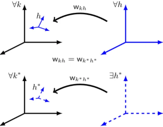
AxSPR: For everyk, k∗, h∈IOb, there existsh∗∈IObsuch thatwkh =wk∗h∗, that is, given observersk, k∗, h, there must (potentially) be someh∗which is related tok∗ in exactly the same way thathis related tok, i.e. the geometrical structure of spacetime cannot forbid such an observer.
In contrast, isotropy refers to the weaker constraint that there is no distin- guished direction in space, i.e. no matter which direction we face, we should be able to perform the same experiments and observe the same outcomes. Isotropy can be expressed in much the same way as SPR, except that we only require equiv- alence as to what can be observed (h) when the relevant observers (kand k∗) are related via a spatial rotation (see Figure 1):
AxIsotropy: For every k, k∗, h ∈ IOb, if wkk∗ ∈ SRot, there exists h∗ ∈ IOb such thatwkh =wk∗h∗.
In order to investigate these ideas, we will need to consider various sets of world- view transformations, and attempt to establish both their algebraic properties and
7This can be expressed in our formal language without any assumption about the structure of quantities as:R(~x)2R(~y)3R(~z)4+R(~x)4R(~y)2R(~z)3+R(~x)3R(~y)4R(~z)2> R(~x)4R(~y)3R(~z)2+ R(~x)2R(~y)4R(~z)3+R(~x)3R(~y)2R(~z)4, hereR(~p)2,R(~p)3, andR(~p)4 denotes the second, third and fourth component ofR(~p)∈Q4, i.e. ifR(~p) = (t, x, y, z), thenR(~p)2 =x,R(~p)3 =y, and R(~p)4=z.
8The quantification over T inAxRelocate appears at first sight to be second-order. How- ever, because translations are determined by the image of the origin, while spatial rotations are determined by the images of the three spatial unit vectors, this axiom can be formalized in our first-order logic language by quantifying over the 4 parameters representing the image of the origin and the 12 parameters representing the images of the three spatial unit vectors.
∀k h
∀h
∀k∗ h∗
∃h∗ wkh
wk∗h∗
wkh=wk∗h∗
Figure 1. Isotropy and the special principle of relativity. The special principle, AxSPR, says that given any k, h and k∗, there exists an h∗ that is related to k∗ the same way that his related to k (i.e. there are no distinguished inertial coordinate systems).
Spatial isotropy,AxIsotropy, is similar, except that we only require h∗to exist whenwkk∗ is a spatial rotation (i.e. rotating ones spatial coordinate system has no effect on what can and cannot potentially be seen).
the relationships between them. The setWk of worldview transformations associ- ated with a specific observerk∈IOb will be defined by
Wk def={wkh :h∈IOb}
and the set ofall worldview transformations is then given by Wdef={wkh :k, h∈IOb}=[
{Wk :k∈IOb}.
W
kk b
a
c
a
b
c wka
wkb
wkc
. . .
Figure 2. The set Wk of all worldview transformations intok’s coordinate system. For each observer a, b, c, . . ., the set Wk con- tains the associated transformationwka,wkb,wkc, . . ..
Using these notations AxSPR can be reformulated as saying that all inertial observers have essentially the same worldview, i.e.Wk =Wk∗ for all k, k∗ ∈IOb.
Although it is not immediately obvious that anyWkcan form a group, if we assume AxWvt it can be proven that AxSPR is equivalent to saying that there is at least onek for whichWk forms a group under composition, which is itself equivalent to saying that Wk =W. For the proof of this and other equivalent formulations of AxSPR, see [MSS19, Prop. 2.1]. Similarly,AxIsotropyis equivalent to saying, for all k, k∗∈IOb, ifwkk∗ ∈SRot, thenWk=Wk∗.
Remark 4.1. We have already noted thatAxSPR entails AxIsotropy, so that the special principle of relativity is at least as strong assumption as spatial isotropy. In fact, it is strictly stronger, becauseWis a group in all models ofKIN+AxIsotropy, but Wk need not be. In particular, therefore, KIN+AxIsotropy does not imply AxSPR. This remains true even if we add the restriction that (Q,+,·,0,1,≤) is the ordered field of real numbers. However, if we add the assumption that co-located observers agree on the direction of time, then it can be shown thatKIN+AxIsotropy impliesAxSPR.
For easy reference, Table 1 summarizes the axioms used in this paper and dis- cussed above.
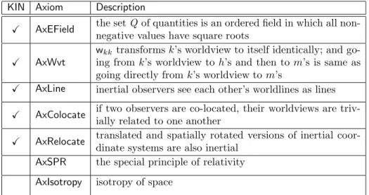
Table 1. Our axioms and their intuitive meanings.
KIN Axiom Description
X AxEField the setQ of quantities is an ordered field in which all non- negative values have square roots
X AxWvt
wkktransformsk’s worldview to itself identically; and go- ing fromk’s worldview toh’s and then to m’s is same as going directly fromk’s worldview tom’s
X AxLine inertial observers see each other’s worldlines as lines X AxColocate if two observers are co-located, their worldviews are triv-
ially related to one another
X AxRelocate translated and spatially rotated versions of inertial coor- dinate systems are also inertial
AxSPR the special principle of relativity AxIsotropy isotropy of space
5. Main theorems
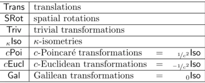
First let us introduce the transformations that will be used in this paper to char- acterize the worldviews of observers. In this section, we assume that (Q,+,·,0,1) is a field. Table 2 summarizes the various transformation groups referred to in the theorems.
5.1. κ-isometries. Given~p = (t, x, y, z), the(squared) κ-length of~p is defined by
k(t, x, y, z)k2κ
def=t2−κ(x2+y2+z2), or in other words,
k~pk2κ
def=~p2t−κ|~ps|2.
Table 2. Transformation groups considered in this paper.
Trans translations SRot spatial rotations
Triv trivial transformations
κIso κ-isometries
cPoi c-Poincar´e transformations = 1/c2Iso cEucl c-Euclidean transformations = −1/c2Iso Gal Galilean transformations = 0Iso
Takingκ= 1 gives the squaredMinkowski length k~pk21=t2−(x2+y2+z2) of~p, whileκ=−1 gives its squaredEuclidean length,k~pk2−1=|~p|2=t2+ (x2+y2+z2).
Definition 5.1.1 (κ-isometry, κ6= 0). If κ 6= 0, we call a linear transformation f : Q4 →Q4 a linear κ-isometry provided it preservesκ-length, i.e. for every
~p ∈Q4,
kf(~p)k2κ=k~pk2κ.
In the case ofκ= 0, we require more than simply preserving 0-length, for while 0-length takes account of temporal extent, it ignores spatial structure. We therefore need to add an extra condition to the definition of 0-isometry to ensure that spatial structure is also respected when considering points with equal time coordinates.9 Definition 5.1.2(κ-isometry,κ= 0). Letf :Q4→Q4be a linear transformation.
We callf alinear 0-isometry provided, for every~p ∈Q4, (5.1) f(~p)2t =~p2t and
~pt= 0 ⇒ |f(~p)s|2=|~ps|2 .
We call the composition of a linearκ-isometry and a translation aκ-isometry, and writeκIsofor theset of allκ-isometries.
Definition 5.1.3 (cPoi, cEucl and Gal). For c > 0, 1/c2-isometries will be called c-Poincar´e transformations and −1/c2-isometries will be called c-Euclidean isometries. Parametercinc-Poincar´e transformations corresponds to the “speed of light”. A 0-isometry is also called aGalilean symmetry. We denote these sets of transformations bycPoi,cEuclandGal, respectively.
It is easily verified that each of these sets forms a group under function compo- sition. In general, when we speak about a setGof transformations as a group, we meanGunder function composition, i.e. (G,◦). As usual, we writeH≤Gto mean thatHis a subgroup ofG, andH<Gto mean that the inclusion is proper.
We note that 1-Poincar´e transformations form the usual groupPoi of Poincar´e transformations and 1-Euclidean isometries form the usual groupEuclof Euclidean isometries. Notice also that trivial transformations, translations and spatial rota- tions areκ-isometries for all values ofκ. Moreover, by Lemma 6.3.2 (Triv=T
κIso), (5.2) Trans∪SRot⊂Triv= \
κ∈Q
κIso=xIso∩yIso
for any two distinctx, y ∈Q. It follows immediately that Trans∪SRot⊂ cPoi∩ cEucl∩Gal.
9Although every 0-isometry preserves 0-length, the converse is not true.
5.2. The theorems. Our first result, Theorem 5.1 (Characterisation), tells us that if space is isotropic then all worldview transformations are κ-isometries for some κ, and shows how to calculate the value ofκin the case that two observers can be found which move relative to one another.
Theorem 5.1(Characterisation). AssumeKIN+AxIsotropy. Then there is aκ∈Q such that the set of worldview transformations is a set ofκ-isometries, i.e.
W⊆κIso.
In other terms,
either W⊆cPoi,W⊆Gal, orW⊆cEuclfor some c >0.
Moreover,
• if¬∃MovingIObis assumed, thenW⊆Triv;
• if∃MovingIObis assumed, thisκis uniquely determined by thewmk-images of~o and~t where m and k are observers moving relative to one another, and can be calculated as
κ=
wmk ~t
t−wmk(~o)t2−1 wmk ~t
s−wmk(~o)s2 .
For all positive c ∈ Q, the groupcPoi is isomorphic to groupPoi (via natural inner automorphisms of the affine group, representing the effects of changing the spatial or temporal units of measurements) and similarly groupcEuclis isomorphic to the Euclidean transformation groupEucl(via the same inner automorphisms); see [MSS19, Prop. 6.9]. So essentially there are only three nontrivial cases: either all the worldview transformations are relativistic; all of them are classical; or all of them are Euclidean isometries. Subject to this constraint, however, Theorem 5.3 (Model Construction) says that all ‘reasonable’ transformation groups (groups containing the translations and spatial rotations, which we know must be present) can occur as the group of worldview transformations in a model ofKIN+AxSPR.
To present a general model construction, let us writeSym(Q4) for the set of all permutations of Q4. Given any transformation groupG ≤Sym(Q4), we define a model MG of our language by takingIOb:=G andwmk :=m◦k−1 fork, m∈G.
Theorem 5.2 (Satisfaction) connects the axioms ofKINto properties ofG.
Theorem 5.2 (Satisfaction). LetG≤Sym(Q4). Then (a) MG satisfiesAxWvt, AxSPRandW=G.
(b) MG satisfiesAxRelocateiffSRot∪Trans⊆G.
(c) MG satisfiesAxLineiffg[t] is a line for allg∈G.
(d) MG satisfiesAxColocateiffg∈Trivwheneverg∈Gandg[t] =t.
Theorem 5.3 (Model Construction). Assume AxEField. Let G be a group such that
• SRot∪Trans⊆G≤cPoi for somec∈Q; or
• SRot∪Trans⊆G≤cEuclfor somec∈Q; or
• SRot∪Trans⊆G≤Gal.
ThenMG is a model ofKIN+AxSPR for whichW=G.
By Theorem 5.1 (Characterisation), Theorem 5.3 (Model Construction) and The- orem 5.2 (Satisfaction), in order to determine whether a group of symmetries has to be a subgroup of one of the groupscPoi,cEuclandGal, it is sufficient to consider its members’ actions ont:
Theorem 5.4 (Determination). Let (Q,+,·,0,1,≤) be a Euclidean field, and let Gbe a group satisfyingSRot∪Trans⊆G≤Sym(Q4). Then
(i) For allg∈G,g[t] is a line, and
ifg[t] =t, theng∈Triv. ⇐⇒ (ii)G≤cPoi,G≤cEuclorG≤Gal for some positivec∈Q. Our next result, Theorem 5.5 (Classification), tells us that we can classify all possible models by looking at how observers’ clocks run relative to one another.
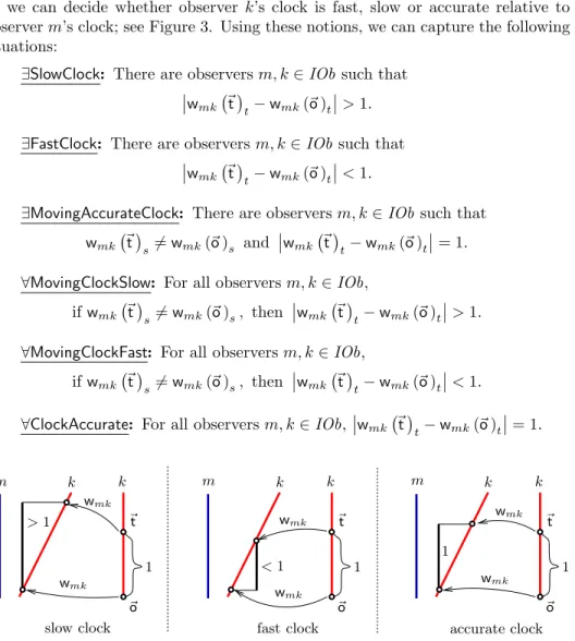
Based on the difference between the time components of the wmk-image of~t and
~o, we can decide whether observer k’s clock is fast, slow or accurate relative to observerm’s clock; see Figure 3. Using these notions, we can capture the following situations:
∃SlowClock: There are observersm, k∈IOb such that wmk ~t
t−wmk(~o)t>1.
∃FastClock: There are observersm, k∈IOb such that wmk ~t
t−wmk(~o)t<1.
∃MovingAccurateClock: There are observersm, k∈IOb such that wmk ~t
s6=wmk(~o)s and wmk ~t
t−wmk(~o)t= 1.
∀MovingClockSlow: For all observersm, k∈IOb, ifwmk ~t
s6=wmk(~o)s, then wmk ~t
t−wmk(~o)t>1.
∀MovingClockFast: For all observersm, k∈IOb, ifwmk ~t
s6=wmk(~o)s, then wmk ~t
t−wmk(~o)t<1.
∀ClockAccurate: For all observersm, k∈IOb,wmk ~t
t−wmk(~o)t= 1.
PSfrag replacements
~o
~o ~o
~t
~t ~t
m
m k k m k k k k
wmk
wmk
wmk
wmk
wmk
wmk
1
1 1
>1
<1
1
slow clock fast clock accurate clock
Figure 3. k’s clock can be fast, slow or accurate according tom
Theorem 5.5 (Classification). Assume KIN+AxIsotropy. Then precisely one of the following four cases holds:
(1) There exists a slow clock (∃SlowClock). In this case, there exists a moving observer (∃MovingIOb), all moving clocks are slow (∀MovingClockSlow), and
W⊆cPoi for some positivec∈Q.
(2) There exists a fast clock (∃FastClock). In this case, there exists a moving observer (∃MovingIOb), all moving clocks are fast (∀MovingClockFast), and
W⊆cEuclfor some positivec∈Q.
(3) There exists a moving accurate clock (∃MovingAccurateClock). In this case, all clocks are accurate (∀ClockAccurate) and
W⊆Gal.
(4) There are no moving observers (¬∃MovingIOb). In this case, W⊆Triv.
By Theorem 5.6 (Consistency), all of these situations can indeed arise.
Theorem 5.6(Consistency). The following axiom systems are all consistent (they all have models):
(1) KIN+AxSPR+∃SlowClock, (2) KIN+AxSPR+∃FastClock,
(3) KIN+AxSPR+∃MovingAccurateClock, (4) KIN+AxSPR+¬∃MovingIOb.
6. Subsidiary theorems and lemmas
Because we use only a small number of basic axioms, we have a large number of intermediate lemmas to prove before we can prove our main theorems. This section is accordingly split into six subsections, each focussing on a key stage in the overall proof of our main findings. Each stage builds on its predecessor(s) and together they establish the following subsidiary theorems. Informally stated, they assert (subject to various conditions) that:
Theorem 6.1 (Observer Lines Lemma):
If ℓ is a possible worldline, then all lines of the same slope as ℓ are also possible worldlines.
Theorem 6.2 (Line-to-Line Lemma):
Each worldview transformation is a bijection taking lines to lines, planes to planes and hyperplanes to hyperplanes.
Theorem 6.3 (tx-Plane Lemma):
Ifwkm maps thetx-plane to itself, then it also maps theyz-plane to itself;
moreover, if wkm is linear, there is some positiveλsuch that |wkm(~p)|= λ|~p|for all~p in theyz-plane.
Theorem 6.4 (Same-Speed Lemma):
Suppose at least one observer considersh andk to be travelling with the same speed. Thenwhk is aκ-isometry for someκ.
Theorem 6.5 (Fundamental Lemma):
Suppose no observers move with infinite speed, and thatspeedk(m) =u >
0. Then there existsε >0 for which, given any positive v≤u+ε, there is somehwithspeedk(h) =vandspeedm(h) =speedm(k).
Theorem 6.6 (Main Lemma):
There exists at least one observer k and one κ for which all worldview transformations wmk involving observers m who agree with k about the origin areκ-isometries.
The order of implications in the proofs that follow is:
Same-Speed
$$
❏❏
❏❏
❏❏
❏❏
❏❏
❏❏
Observer
Lines //Line-to-Line //tx-Plane
99
rr rr rr rr rr rr r
&&
▲▲
▲▲
▲▲
▲▲
▲▲
▲▲
▲ Main
Fundamental
99
tt tt tt tt tt tt
6.1. Observer Lines Lemma. We say that a subsetℓ⊆Q4 is anobserver line for k if there is some observer h for which ℓ = wlk(h), and write ObLines(k) for the set ofk-observer lines. We say thatℓ is anobserver line if there is some kfor which it is an observer line. ByAxLine, all observer lines are lines (because they are worldlines). In this section, we prove that ifk can see an observer travelling along a worldline, then every other line with the same slope is also a worldline as far as kis concerned; there are none of these lines from which observers are banned.
Now supposeAxEFieldholds. Ifℓis a line and~p,~q are distinct points inℓ, we define itsslope by
slope(ℓ)def=
(|~ps−~qs|/|~pt−~qt| if~pt6=~qt,
∞ otherwise .
Theorem 6.1 (Observer Lines Lemma). Assume AxEField, AxWvt, AxRelocate, AxLineandAxIsotropy. Suppose either
(a) slope(ℓ) =slope(ℓ′)6=∞; or else
(b) slope(ℓ) = slope(ℓ′) = ∞ and there exist~p ∈ ℓ and~q ∈ ℓ′ whose time coordinates are equal.
Then for any observerk, we haveℓ∈ObLines(k) iffℓ′ ∈ObLines(k).
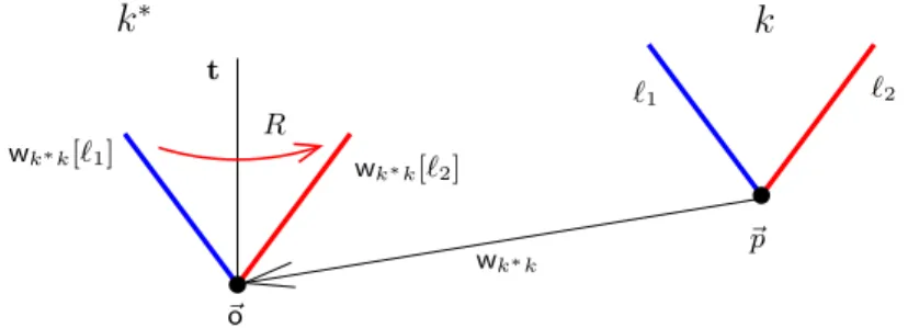
In order to prove this result, we require various supporting lemmas (the more elementary ones are re-used in subsequent proofs). These lemmas refer to a concept we callF-transformationthat relates the worldviews of any two observers via that of a third (see Figure 4). To illustrate the concept, suppose that I am observing two planets,k and k∗, in the night sky. From my point of view, people living on those planets would see the world quite differently, but they nonetheless see the same world I do, so I ought to be able to find some function (F) that transforms
“what I think ksees” into “what I think k∗ sees”. From my point of view, I can say that “k∗ is an ‘F-transformed’ version ofk.”
Definition 6.1.1(F-transforms). Given any bijectionF :Q4→ Q4, we say that k∗ is an F-transformedversion of kaccording toh, and writek Fhk∗if
(6.1) whk∗ =F◦whk.
Remark 6.1. AssumingAxWvt,k Idhk∗ is equivalent to wk∗k=Id, in particular k Idh k; relations k Fh k∗ and k∗ Gh k′ imply k G◦Fh k′; andk Fh k∗ implies k∗F−1hk.
PSfrag replacements
worldview ofh
F
F whk∗
whk
k k∗
whk∗
whk
Worldline Relocation
k Rhk∗ k Fhk∗
wlh(k) wlh(k∗)
Observer Relocation
∃k∗
∀R
∀k
∀h
Figure 4. F-transforms (left) describe how h can transform what it considers to bek’s worldview — and worldline (middle) — into k∗’s (Definition 6.1.1, Lemma 6.1.3 (Worldline Relocation)).
Lemma 6.1.4 (Observer Rotation) tells us that all spatial rotations can be interpreted asF-transforms (right).
6.1.1. Supporting lemmas. Some of these initial lemmas are quite elementary, but they form the bedrock of what follows, and we need to prove them formally to ensure they definitely follow from our somewhat restricted first-order axiom set.
The supporting lemmas can be informally described as follows:
Lemma 6.1.2 (WVT):
This describes various elementary properties concerning worldview trans- formations. We often use these results without further mention.
Lemma 6.1.3 (Worldline Relocation):
IfhcanF-transformkintok∗, then that transformation mapsk’s worldline intok∗’s.
Lemma 6.1.4 (Observer Rotation):
Every spatial rotation can be interpreted as anF-transform.
Lemma 6.1.5 (Transformed Observer Lines):
Ifℓis an observer line fork, thenwhk[ℓ] is an observer line forh.
Lemma 6.1.6 (Rotated Observer Lines):
Ifℓis an observer line fork, so is any spatially rotated copy of ℓ.
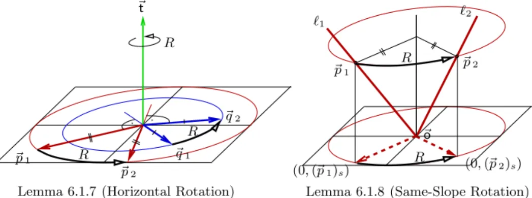
Lemma 6.1.7 (Horizontal Rotation):
This is a technical lemma telling us when one pair of mutually orthogonal horizontal vectors can be spatially rotated into another (where “horizontal”
means “orthogonal to the time-axis”).
Lemma 6.1.8 (Same-Slope Rotation):
If two lines have the same slope and both pass through the origin, it is possible to spatially rotate one into the other.
Lemma 6.1.9 (Observer Line Intersections):
Suppose two intersecting lines have the same slope. If one of them is an observer line fork, then so is the other.
Lemma 6.1.10 (Triangulation):
Suppose t′ is a line parallel to the time-axis, t, and that~p is not on t′. Given any positiveλwe can find linesℓ1 andℓ2which intersect at~p, meet t′ at different points, and have the same slope, λ. In other words, we can find an isosceles triangle whose base is alongt′ and vertex at~p, and whose equal non-base sides both have slopeλ.
6.1.2. Proofs of the supporting lemmas.
Lemma 6.1.2 (WVT). Assume AxWvt. Then, for everyk, h, m∈IOb, (i) wlk(k) =t;
(ii) whk[wlk(m)] =wlh(m);
(iii) whk :Q4→Q4is a bijection fromQ4 onto itself;
(iv) w−1hk =wkh.
Proof. (i)wlk(k) =wkk[t] =Id[t] =t.
(ii) Since wlk(m) = wkm[t], we have whk[wlk(m)] = whk[wkm[t]] = whm[t] = wlh(m), as required.
(iii), (iv): It follows fromwkh◦whk =wkk =Idandwhk◦wkh =whh=Id that wkh andwhk are mutual inverses, and hence that they are both bijections.
Lemma 6.1.3 (Worldline Relocation). AssumeAxWvt, and supposek Fh k∗ for some bijectionF :Q4→Q4. ThenF mapswlh(k) ontowlh(k∗); see Fig. 4 (middle).
Proof. Recall thatk Fhk∗ meanswhk∗ =F◦whk. So
wlh(k∗) =whk∗[t] = (F◦whk) [t] =F[wlh(k)].
Lemma 6.1.4 (Observer Rotation). Assume AxEField, AxWvt, AxRelocate and AxIsotropy. Then given any spatial rotationR∈SRotandk, h∈IOb, there exists an observerk∗ such thatk Rhk∗; see Fig. 4 (right).
Proof. ByAxRelocate, there exists an observerh∗ for whichwhh∗ =R. Becauseh andh∗ are related via a spatial rotation, AxIsotropy tells us there existsk∗∈IOb which is related toh∗ the same way kis related toh, i.e.wh∗k∗ =whk. It follows immediately thatwhk∗ =whh∗ ◦wh∗k∗ =R◦whk, i.e.k Rhk∗, as claimed.
Lemma 6.1.5(Transformed Observer Lines). AssumeAxWvt. Thenℓ∈ObLines(k) iffwhk[ℓ]∈ObLines(h).
Proof. This follows immediately from Lemma 6.1.2 (WVT), since all k-observer
lines are worldlines.
Lemma 6.1.6 (Rotated Observer Lines). Assume AxEField, AxWvt, AxRelocate and AxIsotropy. If ℓ ∈ ObLines(k) and R ∈ SRot is any spatial rotation, then R[ℓ]∈ObLines(k).
Proof. Chooseh∈IObsuch thatℓ=wlk(h). By Lemma 6.1.4 (Observer Rotation), there is someh∗∈IOb for whichh Rk h∗, i.e. wkh∗ =R◦wkh. By Lemma 6.1.3 (Worldline Relocation), we have thatwlk(h∗) =R[wlk(h)] =R[ℓ], and this worldline
is inObLines(k), as required.
Lemma 6.1.7 (Horizontal Rotation). Let (Q,+,·,0,1,≤) be an ordered field and suppose~p1,~q1,~p2,~q2∈Q4satisfy:
(a) ~p1 and~p2have the same length, as do~q1and~q2:
|~p1|2=|~p2|2and|~q1|2=|~q2|2;
(b) ~p1 and~q1 are horizontal and mutually orthogonal:
~p1·~t =~q1·~t =~p1·~q1= 0; and
(c) ~p2 and~q2 are horizontal and mutually orthogonal:
~p2·~t =~q2·~t =~p2·~q2= 0.
Then there exists a spatial rotationR∈SRotsuch thatR(~p1) =~p2andR(~q1) =
~q2; see the left-hand side of Figure 5.
PSfrag replacements
~t
~p1
~p1
~p2 R
R R
R
~q1 R
~q2
Lemma 6.1.7 (Horizontal Rotation)
ℓ1 ℓ2
(0,(~p1)s) (0,(~p2)s)
~o
Lemma 6.1.8 (Same-Slope Rotation)
~p2
Figure 5. Illustrations for Lemma 6.1.7 (Horizontal Rotation) and Lemma 6.1.8 (Same-Slope Rotation).
Proof. Consider the linear map that takesα~t+β~p1+γ~q1toα~t+β~p2+γ~q2. It is easy to see that this map is a linear Euclidean isometry between two subspaces of Q4 which are each at most three-dimensional. Hence, by the refinement of Witt’s theorem [ST71, Thm 234.1, p.234] there is an extensionR :Q4 →Q4 which is a linear Euclidean isometry with determinant 1. ThisR must be a spatial rotation,
becauseR(~t) =~t.
Lemma 6.1.8 (Same-Slope Rotation). Let (Q,+,·,0,1,≤) be a Euclidean field.
Assume ℓ1 andℓ2are lines such that slope(ℓ1) =slope(ℓ2) and~o ∈ℓ1∩ℓ2. Then there existsR∈SRotsuch thatR[ℓ1] =ℓ2.
Proof. Let~p1∈ℓ1and~p2∈ℓ2be such that~p16=~o 6=~p2and (~p1)t= (~p2)t, see the right-hand side of Figure 5. Then|(0,(~p1)s)|2=|(0,(~p2)s)|2. Taking~q1=~q2=~o, Lemma 6.1.7 (Horizontal Rotation) now tells us there exists a spatial rotation R that takes (0,(~p1)s) to (0,(~p2)s) and leaves~o fixed. Since spatial rotations leave time coordinates unchanged, thisRtakes~p1to~p2, and since it also fixes the origin
it must takeℓ1toℓ2.
Lemma 6.1.9 (Observer Line Intersections). Assume AxEField, AxWvt, AxLine, AxRelocate, andAxIsotropy. If two linesℓ1, ℓ2intersect one another and have equal slope, then for anyk∈IOb we haveℓ1∈ObLines(k) iffℓ2∈ObLines(k).
PSfrag replacements
t
~o
~p wk∗k
ℓ1 ℓ2
wk∗k[ℓ2] wk∗k[ℓ1]
k
∗k
R
wk∗k
Figure 6. Illustration for the proof of Lemma 6.1.9 (Observer Line Intersections).
Proof. Let~p be the point of intersection ofℓ1 andℓ2, and letT be the translation taking~p to the origin,~o. By AxRelocate, there exists somek∗ ∈ IOb such that wk∗k =T; see Figure 6.
Note first that the images ofℓ1andℓ2underwk∗kare lines of equal slope because wk∗k = T is a translation, and translations map lines to lines and leave slopes unchanged. Moreover, both of these lines pass throughT(~p) =~o, so Lemma 6.1.8 (Same-Slope Rotation) tells us there exists a spatial rotationRtaking wk∗k[ℓ1] to wk∗k[ℓ2].
The claim now follows. For suppose ℓ1 is a k-observer line; we have to show that ℓ2 is also a k-observer line. Since wk∗k[ℓ1] ∈ ObLines(k∗) by Lemma 6.1.5 (Transformed Observer Lines), it follows that wk∗k[ℓ2] ∈ ObLines(k∗) as well, by Lemma 6.1.6 (Rotated Observer Lines). Applying Lemma 6.1.5 (Transformed Ob- server Lines) in the opposite direction now tells us thatℓ2∈ObLines(k), as required.
The converse follows by symmetry.
Lemma 6.1.10(Triangulation). AssumeAxEField. Lett′ be a line parallel to the time-axis and let~p be any point not on t′. Given any positive λ∈Q, there exist linesℓ1, ℓ2 with
(i) slope(ℓ1) =slope(ℓ2) =λ, (ii) ~p ∈ℓ1∩ℓ2,
(iii) ℓ1∩t′ 6=∅, (iv) ℓ2∩t′ 6=∅,
(v) ℓ1∩ℓ2∩t′=∅.
PSfrag replacements
t′ ℓ1
ℓ2
~p ~q
~q1
~q2
Proof. Let~q ∈t′ be the point ont′ with~qt=~pt. We know that~ps6=~qs because
~p 6∈t′. Consider the points
~q1:=~q + (|~ps−~qs|/λ,0,0,0) and ~q2:=~q −(|~ps−~qs|/λ,0,0,0) and letℓ1be the line passing through~p and~q1, andℓ2 the line passing through~p and~q2. Then direct calculation shows thatℓ1andℓ2 have the required properties.
6.1.3. Main proof. We now complete the proof of Theorem 6.1 (Observer Lines Lemma).
We use the word plane in the usual Euclidean sense to mean a 2-dimensional slice of Q4, and refer to 3-dimensional ‘slices’ as hyperplanes. Formally, a subset P ⊆Q4 is a plane iff there are linearly independent vectors~v , ~w 6=~o ∈Q4 and a point ~p ∈ Q4, such that P = {~p +λ~v +µ~w : λ, µ ∈ Q} (hyperplanes are defined analogously). By AxEField, the usual properties of Euclidean planes hold.
In particular, a planeP can be specified by giving a lineℓ⊆P and a point~p ∈P\ℓ, or three distinct non-collinear points~p ,~q ,~r ∈ P, or two distinct but intersecting lines in P. Moreover, given a line ℓ ⊆P and a point~p ∈ P\ℓ, there is exactly one lineℓp through~p that is parallel toℓ (indeed, if we assumeAxEField, the way in which we have defined line andplane allows us to uniquely determineℓp in the usual way once~p andℓ are specified).
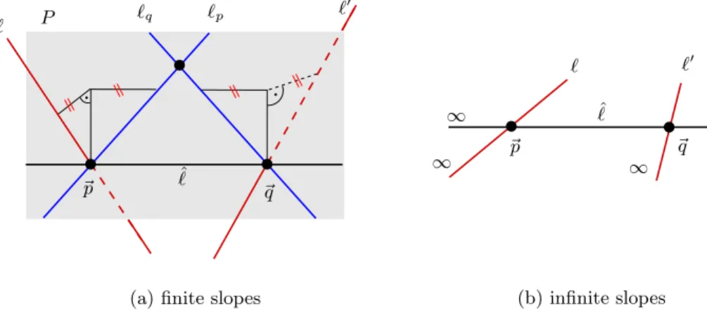
Proof of Theorem 6.1 (Observer Lines Lemma). Let ℓ, ℓ′ be lines of equal slope:
slope(ℓ) = slope(ℓ′). If ℓ = ℓ′, there is nothing to prove, so assume that ℓ 6=ℓ′. Also, if slope(ℓ) = slope(ℓ′) = 0, then ℓ and ℓ′ are both parallel to the time-axis, and it follows easily fromAxRelocatethatℓ, ℓ′∈ObLines(k).
Suppose, therefore, thatslope(ℓ) =slope(ℓ′)6= 0.
Note first that there exist~p ,~q ∈Q4 such that
~p ∈ℓ, ~q ∈ℓ′, ~p 6=~q , and ~pt=~qt.
This is true by assumption for case (b), whereslope(ℓ) =slope(ℓ′) =∞, and it is easy to see that such~p ,~q also exist in case (a) whereslope(ℓ) =slope(ℓ′) is finite.10 Let ˆℓbe the line containing~p and~q. Because~p ,~q have the same time coordinate, slope(ˆℓ) =∞; see Figure 7.
PSfrag replacements
P ℓq ℓp
ℓ
ℓ ℓ′
ℓ′
~p
~p ~q
∞ ∞ ~q
(a) finite slopes (b) infinite slopes
ℓˆ
ℓˆ
∞
Figure 7. Illustration for the proof of Theorem 6.1 (Observer Lines Lemma)
We now consider cases (a) and (b) in turn.
10Pick any point~p onℓthat isn’t onℓ′ and consider the ‘horizontal time slice’ containing it;
becauseℓ′has finite slope, it must also pass through this time slice. Take~qto be the corresponding point of intersection onℓ′.
Case (a): finite slopes. By assumption, 0 < slope(ℓ) = slope(ℓ′) 6= ∞ and slope(ˆℓ) =∞. LetP be the plane containing ˆℓand parallel to t.11
Lettp be the line parallel totwhich passes through~p, and notice that this line lies in P. Choose any point~p′ ∈ P \tp and let λ = slope(ℓ) = slope(ℓ′). Then Lemma 6.1.10 (Triangulation) tells us that we can find two distinct lines which pass through~p′, lie in P (because they meet both~p′ and tp), and have slope λ.
Applying the translation taking~p′to~p, the images of those two lines will still lie in P and still have slopeλ, but will intersect at~p. Similarly, we can find two distinct lines of slope λ which lie inP and pass through~q. Pick one of the lines passing through~q, and call itℓq. Since the two lines through~p are distinct, they cannot both be parallel to ℓq — letℓp be one that isn’t. Sinceℓp andℓq are non-parallel lines lying in the same plane, they must intersect.
The claim now follows. For supposeℓ∈ObLines(k). Thenℓand ℓp are lines of equal slope which intersect at~p, so Lemma 6.1.9 (Observer Line Intersections) tells us that ℓp is also inObLines(k), whence (applying the same argument twice more) so areℓq (because it meetsℓp) andℓ′ (since it meetsℓq).
Case (b): infinite slopes. If slope(ℓ) =∞, thenℓ and ˆℓare two lines of infinite slope which intersect at~p. Likewise,ℓ′ and ˆℓare lines of infinite slope that intersect at~q. As before it now follows by Lemma 6.1.9 (Observer Line Intersections) that
ℓ∈ObLines(k)⇐⇒ℓˆ∈ObLines(k)⇐⇒ℓ′ ∈ObLines(k).
In both cases, therefore, we have ℓ ∈ ObLines(k) ⇐⇒ ℓ′ ∈ ObLines(k), as re-
quired.
6.2. Line-to-Line Lemma.
Theorem 6.2(Line-to-Line Lemma). AssumeAxEField,AxWvt,AxLine,AxRelocate, AxIsotropyand∃MovingIOb. Then given anyk, h∈IOb, the worldview transforma- tionwhk is a bijection that takes lines to lines, planes to planes, and hyperplanes to hyperplanes.
6.2.1. Supporting lemmas. A number of the supporting lemmas refer to the concept of anobserver line triad:
Definition 6.2.1(Observer Line Triads). Ifℓ1, ℓ2, ℓ3∈ObLines(k) are three (nec- essarily coplanar) lines, each pair of which intersect in a point, and whose pairwise intersections are not collinear, we shall call the set{ℓ1, ℓ2, ℓ3}anobserver line triad
for k, or simply ak-triad.
The lemmas can be described informally as follows:
Lemma 6.2.4 (Speed):
Speeds are well-defined, and the terms at rest and in motion have their expected meanings.
Lemma 6.2.5 (Triads):
If one observer considers that three worldlines form a triad, all other ob- servers agree.
Lemma 6.2.6 (Plane-to-Plane):
Suppose planeP contains ak-triad whose slopes are either all finite or else all infinite. Thenwhk[P] is contained in a plane.
11P is parallel totiffP contains a line parallel tot.
Lemma 6.2.7 (Infinite Speeds⇒ Lines are Observer Lines):
If infinite speeds occur, then all lines are observer lines.
6.2.2. Proofs of the supporting lemmas.
Definition 6.2.2. SupposeAxEFieldandAxLine holds. Ifℓ=wlk(h), we call the slope,slope(ℓ), of lineℓthespeed ofhaccording tok, i.e.
speedk(h)def=slope(wlk(h)).
Definition 6.2.3. Recall that observer k ∈IOb is moving according to observer m ∈ IOb iff wmk(~t)s 6= wmk(~o)s and at rest according to m otherwise. We say thatobserver k∈IOb is moving instantaneously according to observer miff wmk(~t)t=wmk(~o)t.
Lemma 6.2.4 (Speed). Assume AxWvt, AxEField and AxLine. Then for every m, k∈IOb, speedm(k) is well-defined, and
• kis at rest according tomiff speedm(k) = 0,
• kis moving according tomiffspeedm(k)6= 0, and
• kis moving instantaneously according to miffspeedm(k) =∞.
Proof. ByAxEFieldandAxLine, it follows thatspeedm(k) is unambiguously defined for allkandm. The proof is straightforward after noticing thatwmk(~t)6=wmk(~o) which holds becausewmk is a bijection by Lemma 6.1.2 (WVT).
Lemma 6.2.5 (Triads). Suppose AxEField, AxWvt, AxLine. Let k, h ∈ IOb. If T ={ℓ1, ℓ2, ℓ3}is ak-triad, thenwhk[T] :={whk[ℓ1],whk[ℓ2],whk[ℓ3]}is anh-triad.
Proof. Each ℓi is a k-observer line, so by Lemma 6.1.5 (Transformed Observer Lines), eachℓ′i=whk[ℓi] is anh-observer line (and hence a line). Becausewhk is a bijection, we know that any two of the lines inwhk[T] has non-empty intersection, and that they have three distinct pairwise intersections in total. It follows that the three lines are coplanar and that their three pairwise intersection points are not collinear. That is,whk[T] is anh-triad as claimed.
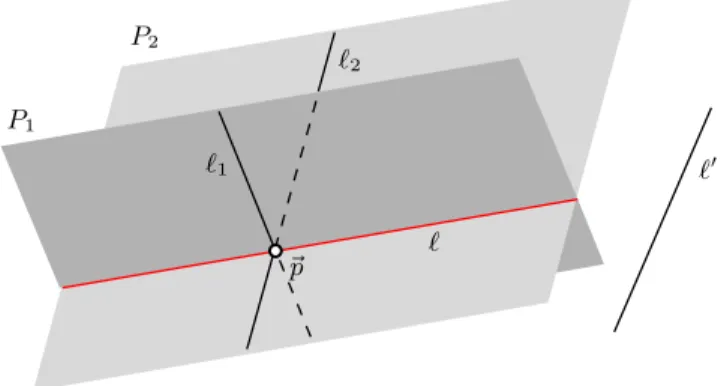
Lemma 6.2.6(Plane-to-Plane). AssumeAxEField,AxWvt,AxLine,AxRelocateand AxIsotropy. Choosek, h∈IOb, letP be a plane which contains ak-triad{ℓ1, ℓ2, ℓ3}, and suppose that the slopes of these lines are either all finite, or else all infinite.
Thenwhk[P] is contained in a plane.
Proof. According to Lemma 6.2.5 (Triads), the lines whk[ℓi] (i = 1,2,3) form an h-triad. We can therefore defineP′, the plane spanned by this triad. We will prove thatwhk[P]⊆P′.
Choose any~p ∈P. If~p lies on any of the linesℓi, then the conclusionwhk(~p)∈ P′ is trivial. Suppose, then, that~p does not lie on any of these lines. Because the lines form a triad we can draw a line ℓ through~p which is parallel to one of the lines (wlog,ℓ1) and which intersects the other two lines (ℓ2and ℓ3) in distinct points.
We claim thatℓ∈ObLines(k). If all three lines have finite slope, this follows from Theorem 6.1 (Observer Lines Lemma) because ℓ and ℓ1 have equal (hence finite) slopes andℓ1is ak-observer line. On the other hand, if all three lines (and hence alsoℓ) have infinite slope, this means there existt1,t2 andt3such that all points on ℓi (i = 1,2,3) have time component ti. But we know that the lines intersect