Thickness distribution of Boolean functions in 4 and 5 variables and a comparison with
other cryptographic properties
Mathias Hopp
a∗, Pål Ellingsen
a, Constanza Riera
a, Pantelimon Stănică
b†aDepartment of Computer Science, Electrical Engineering and Mathematical Sciences,
Western Norway University of Applied Sciences, 5020 Bergen, Norway mathias.hopp@spv.no,{pel,csr}@hvl.no
bApplied Mathematics Department, Naval Postgraduate School, Monterey, USA
pstanica@nps.edu Submitted: September 23, 2020
Accepted: October 20, 2020 Published online: October 29, 2020
Abstract
This paper explores the distribution of algebraic thickness of Boolean functions (that is, the minimum number of terms in the ANF of the func- tions in the orbit of a Boolean function, through all affine transformations), in four and five variables, and the complete distribution is presented. Addi- tionally, a complete analysis of some complexity properties (e.g., nonlinearity, balancedness, etc.) of all relevant orbits of Boolean functions is presented.
Some properties of our notion of rigid function (which enabled us to reduce significantly the computation) are shown and some open questions are pro- posed, providing some further explanation of one of these questions.
Keywords:Boolean function, algebraic normal form, thickness, nonlinearity, affine equivalence
MSC:06E30, 11T06, 94A60, 94D10.
∗Currently with Sparebanken Vest, Bergen, Norway
†Corresponding author 52(2020) pp. 117–135
doi: https://doi.org/10.33039/ami.2020.10.004 url: https://ami.uni-eszterhazy.hu
117
1. Introduction
In this paper, we deal with the concept of algebraic thickness, defined by Carlet in [3, 4] as the minimum number of terms of all Boolean functions in the affine equivalence orbit of a Boolean function – and aim to reveal the distribution of algebraic thickness of all Boolean functions in four and five variables.
As will be discussed in the coming sections, by using an exhaustive search, the calculation of this distribution for 𝑛 ≤ 4 variables is at best a straightforward, and at worst, a lengthy – but manageable – endeavor. There are 22𝑛 Boolean functions in 𝑛 variables, which, for 𝑛= 4, equals 65536. Since there are 322560 different affine transformations needed to be checked for each Boolean function, the calculation of the algebraic thickness for all Boolean functions in four variables is a time consuming task, albeit doable.
However, in moving from four to five variables, this number grows significantly.
The total number of unique Boolean functions is 4 294 967 296, and the number of different affine transformations is 319 979 520. One of the sub-goals of the paper was to find an efficient method able to handle the magnitude of the computation, and another was to effectively handle and analyze the resulting data set for𝑛= 5.
Additionally, throughout the paper, when discussing functions𝑛≤5, we omit the trivial cases𝑛= 0,1, unless specified. We used SageMath [9] for all computa- tions in this paper.
A Boolean function𝑓in𝑛variables, where𝑛is any positive integer, is a function from the vector space F𝑛2 to the finite field F2, i.e. 𝑓: F𝑛2 → F2. The set of all Boolean functions in 𝑛 variables is denoted by ℬ𝑛, and the symbol ⊕ denotes addition modulo 2, inF2,F𝑛2, andℬ𝑛.
Every Boolean function𝑓 has a unique representation called itsalgebraic normal form (ANF) as a polynomial overF2 in𝑛variables:
𝑓(x) = ⨁︁
u∈F𝑛2
𝑐u
(︃ 𝑛
∏︁
𝑖=1
𝑥𝑢𝑖𝑖 )︃
= ⨁︁
u∈F𝑛2
𝑐uxu,
where each 𝑐u∈F2, u= (𝑢1, . . . , 𝑢𝑛) andx= (𝑥1, . . . , 𝑥𝑛). The algebraicdegree of𝑓 is the largest weight of usuch that𝑐u̸= 0. Ahomogeneous function is a sum of monomials of the same degree.
An affine function ℓu,𝑐 is a function with algebraic degree at most 1, which takes the form
ℓu,𝑐(x) =u·x⊕𝑐=𝑢1𝑥1⊕ · · · ⊕𝑢𝑛𝑥𝑛⊕𝑐, (1.1) where u= (𝑢1, . . . , 𝑢𝑛)∈F𝑛2 and𝑐∈F2. If 𝑐= 0, such that ℓu,0 only consists of monomials of algebraic degree 1, and no constant, then it is alinear function. The Hamming weight of a vectorx∈F𝑛2 is denoted by𝑤𝑡(x)and is equal to the number of 1’s in the vectorx. For a Boolean function𝑓onF𝑛2, letΩ𝑓 ={x∈F𝑛2 |𝑓(x) = 1} be the support of 𝑓. The Hamming weight of 𝑓 is then |Ω𝑓|, or equivalently, the weight of the vector of its truth table. The Hamming distance between two
functions𝑓, 𝑔: F𝑛2 → F2, denoted by 𝑑(𝑓, 𝑔), is defined as 𝑑(𝑓, 𝑔) =𝑤𝑡(𝑓 ⊕𝑔). A balancedfunction on𝑛variables has weight exactly2𝑛−1. For𝑓:F𝑛2 →F2we define theWalsh-Hadamard transformto be the integer-valued function
𝒲𝑓(u) = ∑︁
𝑥∈F2𝑛
(−1)𝑓(x)+ux, u∈F𝑛2.
Thenonlinearity 𝒩𝑓 of a function 𝑓 is defined as 𝒩𝑓 = min
𝜑∈𝒜𝑛
𝑑(𝑓, 𝜑)
where𝒜𝑛is the class of all affine functions onF𝑛2. The largest nonlinearity, namely 2𝑛−1−2𝑛2−1is achieved bybentfunctions (they exist for even dimension𝑛) and they have only two values in their Walsh spectrum (the multiset of Walsh coefficients), namely ±2𝑛2. Thesemi-bentfunctions will have three values in their Walsh spec- trum, namely, {0,±2𝑛+22 }, {0,±2𝑛+12 }, for𝑛even, respectively, odd, and they can be balanced, as opposed to bent functions, whose weight can only be2𝑛−1±2𝑛2−1. For these definitions and to know more on Boolean functions, and their cryp- tographic properties, the reader can consult [2, 5].
2. Algebraic thickness
Carlet, in [3], defined algebraic thickness, and discussed lower and upper bounds.
His paper also includes further discussion on the relation that algebraic thickness has with other complexity criteria (e.g., nonlinearity, algebraic degree, etc.). In [4], Carlet improved some of the prior results, and further expanded on the properties of algebraic thickness.
Definition 2.1 ([4]). The algebraic thickness 𝒯(𝑓) of a Boolean function 𝑓 is the minimum number of monomials with non-zero coefficients in the ANF of the functions 𝑓 ∘ 𝒜, where𝒜 ∈ GL(𝑛,F2) (the general affine group). When we want to emphasize the number of variables, we shall write𝒯𝑛(𝑓).
Surely, the algebraic thickness of affine functions is at most 1 [1, 4]. The quadratic functions are also well understood, due to the well-known Dickson’s the- orem (see MacWilliams and Sloane [8], or the simpler version below taken from Boyar and Find [1]).
Theorem 2.2 (Dickson’s Theorem). If 𝑓:F𝑛2 →F2 is a quadratic Boolean func- tion, then there exist an invertible 𝑛×𝑛matrix𝐴,b∈F𝑛2,𝑡≤ 𝑛2, and𝑐∈F2 such that for y=𝐴x+bone of the following two equations holds:
𝑓(𝑥) =𝑦1𝑦2+𝑦3𝑦4+· · ·+𝑦𝑡−1𝑦𝑡+𝑐, or 𝑓(𝑥) =𝑦1𝑦2+𝑦3𝑦4+· · ·+𝑦𝑡−1𝑦𝑡+𝑦𝑡+1. Furthermore 𝐴,b, and𝑐 can be found efficiently.
We also mention that we re-computed (see Table 4) the distribution of nonlin- earities of all functions in 2 ≤𝑛≤5 variables, confirming known results (see, for instance, the paper by Sertkaya and Doğanaksoy [10]).
For Boolean functions in𝑛variables, it is of interest to determine the maximum value possible for the thickness, namely,𝜏𝑛= max𝑓∈ℬ𝑛(𝒯(𝑓)), and specifically, its growth. Surely, we have the trivial upper bound 𝜏𝑛 ≤ 2𝑛, since the maximum number of terms in the ANF of a function in𝑛variables is≤2𝑛.
Regarding the lower bound of the thickness, Carlet showed in [3] that, for every 𝜆 < 12 and positive integer𝑛, the density inℬ𝑛 of the subset
{𝑓 ∈ ℬ𝑛| 𝒯(𝑓)≥𝜆2𝑛}
is greater than1−22𝑛𝐻2(𝜆)−2𝑛+𝑛2+𝑛, where𝐻2(𝑥) =−𝑥log2(𝑥)−(1−𝑥)log2(1−𝑥) is the entropy function, and thereforealmost all Boolean functions have algebraic thickness greater than 𝜆2𝑛. This was improved in [4], showing that almost all Boolean functions have algebraic thickness greater than 2𝑛−1−𝑛2𝑛−12 . The best upper bound on algebraic thickness is still the one in [3], namely,
𝒯(𝑓)≤ 2 32𝑛, which is believed to be improvable.
3. Some theoretical results on thickness
Brute force computation is still possible for 𝑛= 4, but for𝑛= 5we need to find some techniques to reduce the computational time, as it would take thousands of years on a personal computer. The idea is that this new technique may be useful in approaching the thickness distribution computation for 𝑛 = 6 (or at least for some subclass ofℬ6).
For any Boolean function𝑓, we define its orbit or equivalence class as the set of functions{𝑓∘ 𝒜:𝒜 ∈GL(𝑛,F2)}.
Given a Boolean function 𝑓, if𝑓𝑚𝑖𝑛 is an element (not necessarily unique) of its equivalence class with minimum number of terms, then the algebraic thickness of𝑓𝑚𝑖𝑛 is the number of terms in its ANF.
Definition 3.1 (Rigid Boolean functions). We call a Boolean function 𝑓 with 𝒯(𝑓)monomials in its ANF, arigid function. The set of all rigid functions will be denoted by𝒮𝑛.
Thus, a rigid Boolean function cannot be mapped to a function with lower monomial count, through any affine transformation. Furthermore, any Boolean function can be mapped to a rigid function. The reason for this should be clear, but for completion, we state it as a lemma.
Proposition 3.2. Any Boolean function can be mapped to a rigid function, by an affine transformation.
Proof. Given a Boolean function 𝑓 ∈ ℬ𝑛, let 𝑔 be a function in the orbit of 𝑓 (through affine transformations), where the monomial count of𝑔 is equal to𝒯(𝑓).
If 𝑔 is not a rigid function, then 𝑔 does not have the minimum monomial count in its orbit. Suppose ℎ is in the orbit of 𝑔, and has lower monomial count than 𝑔. Since𝑓 maps to𝑔and 𝑔maps toℎ, then by composition of transformations,𝑓 maps to ℎas well. Thus, we reach a contradiction.
Experimentally, it was found that𝒮𝑛⊂ 𝒮𝑛+1, for small values of𝑛, suggesting that perhaps this is true in general, and will be shown next.
Theorem 3.3. All rigid functions in𝑛variables are also rigid functions in(𝑛+ 1) variables, that is,𝒮𝑛 ⊂ 𝒮𝑛+1.
Remark 3.4. As is customary in this area (for easy writing), in the following proof, we disregard the usual linear algebra convention of matrix-vector multiplication and regardxand bboth as a row- and a column vector, when there is no danger of confusion.
Proof. Let𝑓 ∈ 𝒮𝑛 with𝒯(𝑓) =𝑡. We embed𝑓 in 𝑛+ 1variables, and we denote its embedding by𝑓˜, such that𝑓˜(𝑥1, . . . , 𝑥𝑛, 𝑥𝑛+1) =𝑓(𝑥1, . . . , 𝑥𝑛). Let a non-zero affine transformation of the input of 𝑓˜be given by x ↦→ 𝐴˜˜x+b, where𝐴˜ is an (𝑛+ 1)×(𝑛+ 1) matrix and b = (𝑏1. . . , 𝑏𝑛), and x˜ = (𝑥1, . . . , 𝑥𝑛, 𝑥𝑛+1),x = (𝑥1, . . . , 𝑥𝑛). We label the first𝑛rows and𝑛columns in𝐴˜by𝐴and so,
𝐴˜=
⎛
⎜⎝
𝑎1,𝑛+1
𝐴 ...
𝑎𝑛+1,1 · · · 𝑎𝑛+1,𝑛+1
⎞
⎟⎠.
Thus,
𝐴˜˜x+b=
⎛
⎜⎜
⎜⎝
𝐴x+𝑥𝑛+1
⎛
⎜⎝ 𝑎1,𝑛+1
...
𝑎𝑛,𝑛+1
⎞
⎟⎠+
⎛
⎜⎝ 𝑏1
...
𝑏𝑛
⎞
⎟⎠ 𝑎𝑛+1,1𝑥1+· · ·+𝑎𝑛+1,𝑛+1𝑥𝑛+1+𝑏𝑛+1
⎞
⎟⎟
⎟⎠,
and so
𝑓˜( ˜𝐴˜x+b) =𝑓
⎛
⎜⎝𝐴x+𝑥𝑛+1
⎛
⎜⎝ 𝑎1,𝑛+1
...
𝑎𝑛,𝑛+1
⎞
⎟⎠+
⎛
⎜⎝ 𝑏1
...
𝑏𝑛
⎞
⎟⎠
⎞
⎟⎠,
from which our claim is inferred.
In summary, the introduction of𝑥𝑛+1 does not induce any further monomial eliminations not already possible in 𝑛 variables. Therefore, for a rigid function𝑓 with monomial count𝑡,
𝒯𝑛(𝑓) =𝑡=𝒯𝑛+1( ˜𝑓).
Corollary 3.5. For any Boolean function𝑓 in 𝑛variables, 𝒯𝑛(𝑓) =𝒯𝑛+1( ˜𝑓),
where𝑓˜is the embedding of𝑓 in ℬ𝑛+1, such that
𝑓˜(𝑥1, . . . , 𝑥𝑛, 𝑥𝑛+1) =𝑓(𝑥1, . . . , 𝑥𝑛).
Proof. Given a rigid Boolean function 𝑓 in 𝑛variables, let 𝒜𝑛(𝑓) be the orbit of 𝑓 through all nonzero affine transformations, and let 𝒯𝑛(𝑓) = 𝑡. As we know, from the definition of algebraic thickness, any Boolean function𝑔∈ 𝒜𝑛(𝑓)satisfies 𝒯𝑛(𝑔) =𝑡, as well. Since 𝑓 is rigid, 𝒯𝑛+1(𝑓) =𝑡, by Theorem 3.3. Clearly, then, 𝒜𝑛(𝑓)⊆ 𝒜𝑛+1( ˜𝑓), by the very same affine transformations as in𝑛variables (leaving the new variable𝑥𝑛+1mapped to itself), and therefore all functions in𝒜𝑛(𝑓)have thickness𝑡 in𝑛+ 1variables, as well.
3.1. Multiplication by a new variable may conserve thickness
We showed in Theorem 3.3 that all rigid functions inℬ𝑛 are also rigid functions in ℬ𝑛+1. Moreover, 𝑓 ∈ ℬ𝑛, 𝒯𝑛(𝑓) =𝒯𝑛+1( ˜𝑓), as well. These properties give insight into the distribution of algebraic thickness in(𝑛+1)variables, when the distribution for𝑛variables is known. Surely, we cannot expect an inductive procedure for the computation of thickness, but as observed already in Theorem 3.3, a connection does exist that may decrease the complexity even further.
Proposition 3.6. Let 𝑓 ∈ ℬ𝑛 be a Boolean function in variables x= (𝑥1, ..., 𝑥𝑛) vector, and let 𝑥𝑛+1 be a new variable. Then:
𝒯𝑛+1(𝑓(𝑥1, . . . , 𝑥𝑛)·𝑥𝑛+1)≤ 𝒯𝑛(𝑓).
Proof. Given a Boolean function𝑓 ∈ ℬ𝑛, with known algebraic thickness𝒯𝑛(𝑓) =𝑡, on the variables (𝑥1, . . . , 𝑥𝑛), we let𝑓min∈ ℬ𝑛 be the representative function with monomial count𝑡of the orbit of𝑓, and let𝜋denote the affine transformation such that 𝜋(𝑓) =𝑓min. As before,𝑥𝑛+1 is the new variable introduced inℬ𝑛+1.
Inℬ𝑛+1, then, 𝜋′(𝑓(𝑥1, . . . , 𝑥𝑛)·𝑥𝑛+1) =𝑓min(𝑥1, . . . , 𝑥𝑛)·𝑥𝑛+1, by the trans- formation 𝜋′(𝑥𝑗) = 𝜋(𝑥𝑗), for 𝑗 <(𝑛+ 1), and 𝜋′(𝑥𝑛+1) = 𝑥𝑛+1. Since𝑓min has monomial count𝑡,𝑓min(𝑥1, . . . , 𝑥𝑛)·𝑥𝑛+1also has monomial count𝑡, and therefore 𝒯𝑛+1(𝑓(𝑥1, . . . , 𝑥𝑛)·𝑥𝑛+1)≤ 𝒯𝑛(𝑓).
Based upon extensive computations (exhaustive for lower dimensions and ran- dom for higher dimensions) and the previous proposition, we propose the following question.
Open question 3.7 (Thickness conservation). Let 𝑓 ∈ ℬ𝑛 be a Boolean function in variables x= (𝑥1, ..., 𝑥𝑛)vector, and let 𝑥𝑛+1 be a new variable. Is it true that
𝒯𝑛+1(𝑓(𝑥1, . . . , 𝑥𝑛)·𝑥𝑛+1) =𝒯𝑛(𝑓)?
While this is not necessarily the goal of the paper, and we cannot provide an answer to this question, we attempt to explain it further. Assume that there exists a function 𝑓 in 𝑛variables such that 𝒯𝑛(𝑓)>𝒯𝑛+1(𝑓·𝑥𝑛+1) =𝑡. Take an affine transformation that brings𝑓(𝑥1, . . . , 𝑥𝑛)·𝑥𝑛+1to its minimal thickness form, transformation determined by the vectorb= (𝑏1, . . . , 𝑏𝑛+1), and the matrix 𝐴˜ of the form
𝐴˜=
⎛
⎜⎝
𝑎1,𝑛+1
𝐴 ...
𝑎𝑛+1,1 · · · 𝑎𝑛+1,𝑛+1
⎞
⎟⎠, where𝐴 is an𝑛×𝑛matrix, and so,
𝐴˜˜x+b=
⎛
⎜⎜
⎜⎝
𝐴x+𝑥𝑛+1
⎛
⎜⎝ 𝑎1,𝑛+1
...
𝑎𝑛,𝑛+1
⎞
⎟⎠+
⎛
⎜⎝ 𝑏1
...
𝑏𝑛
⎞
⎟⎠ 𝑎𝑛+1,1𝑥1+· · ·+𝑎𝑛+1,𝑛+1𝑥𝑛+1+𝑏𝑛+1
⎞
⎟⎟
⎟⎠,
as in Theorem 3.3. We label 𝑟𝑖,𝐴˜, 𝑟𝑖,𝐴, the 𝑖th row of 𝐴, respectively˜ 𝐴, and x˜= (𝑥1, . . . , 𝑥𝑛, 𝑥𝑛+1),x= (𝑥1, . . . , 𝑥𝑛). Thus, using “·” to denote the usual scalar product,
(𝑓(𝑥1, . . . , 𝑥𝑛)·𝑥𝑛+1)∘( ˜𝐴˜x+b)
=𝑓(𝑟1,𝐴·x+𝑎1,𝑛+1𝑥𝑛+1+𝑏1, . . . , 𝑟𝑛,𝐴·x+𝑎𝑛,𝑛+1𝑥𝑛+1+𝑏𝑛) (3.1)
·(𝑎𝑛+1,1𝑥1+· · ·+𝑎𝑛+1,𝑛+1𝑥𝑛+1+𝑏𝑛+1).
We let 𝑏′𝑖 =𝑏𝑖+𝑎𝑖,𝑛+1𝑥𝑛+1, 1 ≤𝑖 ≤𝑛+ 1 and b′ = (𝑏′1, . . . , 𝑏′𝑛). Since the first factor is simply 𝑓(𝐴x+b′) (we regard its coefficients in F2[𝑥𝑛+1], and assume that 𝐴is invertible; again, it may happen that it is not), it must have more than 𝒯𝑛+1(𝑓(𝑥1, . . . , 𝑥𝑛)·𝑥𝑛+1) =𝑡terms (call them𝑇𝑖(𝑥1, . . . , 𝑥𝑛), of degreesdeg𝑇𝑖= 𝑑𝑖, 1≤𝑖≤𝑠, with𝑑1 ≤𝑑2 ≤ · · · ≤𝑑𝑠), given our assumption. We thus write its algebraic normal form as
𝑓(𝐴x+b′) = (𝛼1𝑥𝑛+1+𝛽1)𝑇1(𝑥1, . . . , 𝑥𝑛) +· · · + (𝛼𝑠𝑥𝑛+1+𝛽𝑠)𝑇𝑠(𝑥1, . . . , 𝑥𝑛), 𝑠 > 𝑡,
(𝛼𝑖, 𝛽𝑖are not zero simultaneously, since we need to have𝑠 > 𝑡terms in𝑓(𝐴x+b′)), and therefore Equation (3.1) becomes (for easy writing, we denote the (𝑛+ 1)st row of𝐴˜by(𝛾1, . . . , 𝛾𝑛+1)and we will not write the input(𝑥1, . . . , 𝑥𝑛)for𝑇𝑖),
∑︁𝑠 𝑖=1
(𝛼𝑖𝑥𝑛+1+𝛽𝑖)𝑇𝑖
⎛
⎝
∑︁𝑛 𝑗=1
𝛾𝑗𝑥𝑗+𝛾𝑛+1𝑥𝑛+1+𝑏𝑛+1
⎞
⎠
=
∑︁𝑛 𝑗=1
∑︁𝑠 𝑖=1
(𝛼𝑖𝑥𝑛+1+𝛽𝑖)𝛾𝑗𝑥𝑗𝑇𝑖(𝑥1, . . . , 𝑥𝑛)
+
∑︁𝑠 𝑖=1
𝛾𝑛+1(𝛼𝑖+𝛽𝑖)𝑥𝑛+1𝑇𝑖+
∑︁𝑠 𝑖=1
(𝛼𝑖𝑥𝑛+1+𝛽𝑖)𝑏𝑛+1𝑇𝑖
=
∑︁𝑠 𝑖=1
𝑥𝑛+1𝑇𝑖
⎛
⎝𝛼𝑖𝑏𝑛+1+𝛾𝑛+1(𝛼𝑖+𝛽𝑖) +𝛼𝑖
∑︁𝑛 𝑗=1
𝛾𝑗𝑥𝑗
⎞
⎠ (3.2)
+
∑︁𝑛 𝑗=1
∑︁𝑠 𝑖=1
𝛽𝑖𝛾𝑗𝑥𝑗𝑇𝑖+
∑︁𝑠 𝑖=1
𝛽𝑖𝑏𝑛+1𝑇𝑖.
=
∑︁𝑠 𝑖=1
⎛
⎝𝛼𝑖𝑏𝑛+1+𝛾𝑛+1(𝛼𝑖+𝛽𝑖) +𝛼𝑖
∑︁𝑛 𝑗=1
𝛾𝑗𝑥𝑗
⎞
⎠𝑥𝑛+1𝑇𝑖
+
∑︁𝑠 𝑖=1
𝛽𝑖
⎛
⎝𝑏𝑛+1+
∑︁𝑛 𝑗=1
𝛾𝑗𝑥𝑗
⎞
⎠𝑇𝑖.
We thus get
(𝑓(𝑥1, . . . , 𝑥𝑛)·𝑥𝑛+1)∘( ˜𝐴˜x+b)
=𝑥𝑛+1
∑︁𝑠 𝑖=1
⎛
⎝𝛼𝑖𝑏𝑛+1+𝛾𝑛+1(𝛼𝑖+𝛽𝑖) +𝛼𝑖
∑︁𝑛 𝑗=1
𝛾𝑗𝑥𝑗
⎞
⎠𝑇𝑖
+
∑︁𝑠 𝑖=1
𝛽𝑖
⎛
⎝𝑏𝑛+1+
∑︁𝑛 𝑗=1
𝛾𝑗𝑥𝑗
⎞
⎠𝑇𝑖.
For the inequality to hold, we need to have enough cancellations in both sums
𝑆1=
∑︁𝑠 𝑖=1
⎛
⎝𝛼𝑖𝑏𝑛+1+𝛾𝑛+1(𝛼𝑖+𝛽𝑖) +𝛼𝑖
∑︁𝑛 𝑗=1
𝛾𝑗𝑥𝑗
⎞
⎠𝑇𝑖
𝑆2=
∑︁𝑠 𝑖=1
𝛽𝑖
⎛
⎝𝑏𝑛+1+
∑︁𝑛 𝑗=1
𝛾𝑗𝑥𝑗
⎞
⎠𝑇𝑖,
for a total of more than(𝑠−𝑡)terms. We let𝐴𝑖 be the index support for𝑇𝑖(that is, if 𝑇𝑖(𝑥1, . . . , 𝑥𝑛) = 𝑥𝑖1· · ·𝑥𝑖ℓ, then 𝐴𝑖 = {𝑖1, . . . , 𝑖ℓ}). Therefore, the above sums can be written as (we let |𝐽|2 =|𝐽| (mod 2), where 𝐽 = {𝑗|𝛾𝑗 ̸= 0}, and
|𝐽𝑖|2=|𝐽𝑖| (mod 2), where 𝐽𝑖={𝑗∈𝐴𝑖|𝛾𝑗̸= 0}),
𝑆1=
∑︁𝑠 𝑖=1
(𝛼𝑖𝑏𝑛+1+𝛾𝑛+1(𝛼𝑖+𝛽𝑖))𝑇𝑖+
∑︁𝑠 𝑖=1
𝛼𝑖
⎛
⎝|𝐽𝑖|2+ ∑︁
𝑗∈𝐽∖𝐽𝑖
𝑥𝑗
⎞
⎠𝑇𝑖
=
∑︁𝑠 𝑖=1
(𝛼𝑖𝑏𝑛+1+𝛾𝑛+1(𝛼𝑖+𝛽𝑖) +𝛼𝑖|𝐽𝑖|2)𝑇𝑖+
∑︁𝑠 𝑖=1
𝛼𝑖𝑇𝑖
∑︁
𝑗∈𝐽∖𝐽𝑖
𝑥𝑗
=
∑︁𝑠 𝑖=1
𝛼𝑖(𝑏𝑛+1+|𝐽𝑖|2)𝑇𝑖+
∑︁𝑠 𝑖=1
𝛼𝑖𝑇𝑖
∑︁
𝑗∈𝐽∖𝐽𝑖
𝑥𝑗+𝛾𝑛+1
∑︁𝑠 𝑖=1
(𝛼𝑖+𝛽𝑖)𝑇𝑖,
𝑆2=
∑︁𝑠 𝑖=1
𝛽𝑖𝑏𝑛+1𝑇𝑖+
∑︁𝑠 𝑖=1
𝛽𝑖
⎛
⎝∑︁
𝑗∈𝐴𝑖
𝛾𝑗+∑︁
𝑗̸∈𝐴𝑖
𝛾𝑗𝑥𝑗
⎞
⎠𝑇𝑖
=
∑︁𝑠 𝑖=1
𝛽𝑖(𝑏𝑛+1+|𝐽𝑖|2)𝑇𝑖+
∑︁𝑠 𝑖=1
𝛽𝑖𝑇𝑖
∑︁
𝑗∈𝐽∖𝐽𝑖
𝑥𝑗.
If𝛾𝑛+1= 0then, for𝑖 such that𝑏𝑛+1+|𝐽𝑖|2 ̸= 0, then either𝛼𝑖(𝑏𝑛+1+|𝐽𝑖|2)𝑇𝑖, or 𝛽𝑖(𝑏𝑛+1+|𝐽𝑖|2)𝑇𝑖 survives. Similarly, assuming that for an𝑖, 𝐽∖𝐽𝑖̸=∅, then either 𝛼𝑖𝑇𝑖∑︀
𝑗∈𝐽∖𝐽𝑖𝑥𝑗, or 𝛽𝑖𝑇𝑖∑︀
𝑗∈𝐽∖𝐽𝑖𝑥𝑗 survives. If it were true that for all 𝑖, 𝐽∖𝐽𝑖 ̸=∅, then the inequality would be false and the conjecture would “hold” in this case. However, at least𝐽∖𝐽𝑠=∅, since otherwise our affinely equivalent function would have degree higher than 𝑑𝑠+ 2(recall that 𝑆1 is multiplied by 𝑥𝑛+1), and that is impossible. If one would attempt to find a counterexample for a negative answer to our open question, then one could take a matrix 𝐴˜ where the last row is rather very sparse, along with𝑏 such that 𝐴x+𝑏′ has most of the𝛽𝑖= 0. Can that be achieved? We do not know the answer to this question.
3.2. Gaps in thickness distribution
Noting the algebraic thickness distributions listed in Table 3, it is easy to see that, for𝑛≤5and𝑚 >0, if there exists a representative with𝒯𝑛=𝑚, then there exists a representative with𝒯𝑛 =𝑚−1, and conversely: if there are no representatives with 𝒯𝑛 =𝑚−1, then there are no representatives with𝒯𝑛 =𝑚. The following conjecture is an extension of Lemma 3.9.
Conjecture 3.8. For any 𝑛, in any given monomial count 𝑚 ≤2𝑛, if there are no rigid functions with𝑚 monomials, then for any𝑓 ∈ ℬ𝑛,
𝒯𝑛(𝑓)< 𝑚.
The idea here is that if there are no rigid functions in a set monomial count 𝑚, then there are no rigid functions in any monomial count 𝑀, where 𝑀 > 𝑚. Proving this would have implications for further attempts at determining maximum algebraic thickness (and the following thickness distribution) using the methods described in this paper, as finding no rigid functions in𝑛variables with monomial count (e.g.) 2𝑛−1 would imply there are no rigid functions with monomial count greater than2𝑛−1, thus eliminating half of the set of functions to search through.
The definition for rigid functions is closely related to Carlet’s definition for algebraic thickness. We record that below.
Proposition 3.9. Given all Boolean functions in𝑛variables with monomial count 𝑘 in their ANF, if there are no rigid functions with𝑘 monomials, then there are no functions 𝑓 in𝑛 variables with𝒯𝑛(𝑓) =𝑘.
This simple proposition was the inception of the program described later to find the thickness distribution.
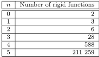
𝑛 Number of rigid functions
0 2
1 3
2 6
3 28
4 588
5 211 259
Table 1: Number of rigid functions in𝑛≤5variables
The distribution of the number of rigid functions in𝑛≤5variables is listed in Table 1, where: for𝑛≤4 variables, these numbers were collected from analysis of the data sets calculated by brute-force, and for𝑛= 5, the number was (along with double-checking values for𝑛 <5) collected from analysis of the data sets calculated by the program described later.
We hope that our methods will prove useful for𝑛 >5, as well, since an itera- tive approach is impossible by modern computing standards for these dimensions.
Searching for rigid functions and – most importantly – disregarding non-rigid func- tions, should improve the efficiency of any program (at the very least, it improves the program given later).
Determining which functions are rigid functions in𝑛variables yields information regarding the thickness distribution in 𝑛+ 1 variables as well, by Theorem 3.3.
Furthermore, by Corollary 3.5, unveiling the distribution of all functions in ℬ𝑛 immediately gives the distribution of22𝑛functions inℬ𝑛+1– which may be a small portion compared to22𝑛+1, but is nonetheless a start.
The functions in𝒮0,𝒮1,𝒮2(i.e., the rigid functions in 𝑛= 0,1,2 variables) are listed below:
𝒮0={0,1} 𝒮1={0,1, 𝑥1}
𝒮2={0,1, 𝑥1,𝑥2,𝑥1𝑥2,𝑥1𝑥2+ 1}
Since the sets 𝒮3,𝒮4 are of rather large sizes (28 and 588, respectively), they will not be listed here (but the data can be found in [7]).
4. Representatives
By uncovering one function𝜑for each of these orbits, every function in𝑛variables can be generated from a corresponding 𝜑, by iteration through all affine trans- formations for each one. Calculating the algebraic thickness of each 𝜑 yields the thickness distribution for all functions inℬ𝑛, as𝒯 is (trivially) an affine invariant.
Since these𝜑would be representing their orbits, the name representative function
𝑛 Number of equivalence classes
1 3
2 5
3 10
4 32
5 382
6 15 768 919
Table 2: Number of affine equivalence classes of Boolean functions [6]
was chosen. As the rigid functions are the functions with the minimum number of monomials in their ANF, these representative functions were chosen to be the smallest rigid functions in their orbit (we call smallest, a function with a minimal sum of the degrees of each monomial in its ANF, with lowest indexed variables, in lexicographical order, in descending order by degree of monomials).
We give an example below.
Example 4.1. For 𝑛 = 3,𝒯3 = 3, and there is a single orbit with maximum thickness, containing9rigid functions, namely: 𝑥1𝑥2𝑥3+𝑥3+ 1,𝑥1𝑥2𝑥3+𝑥2+ 1, 𝑥1𝑥2𝑥3+𝑥1+ 1,𝑥1𝑥2𝑥3+𝑥2+𝑥3,𝑥1𝑥2𝑥3+𝑥1+𝑥3,𝑥1𝑥2𝑥3+𝑥1+𝑥2,𝑥1𝑥2𝑥3+ 𝑥2𝑥3+𝑥1,𝑥1𝑥2𝑥3+𝑥1𝑥3+𝑥2,𝑥1𝑥2𝑥3+𝑥1𝑥2+𝑥3. In the first three functions, the sum of the monomial degrees for each function is 4, the next three functions have this sum 5, and the last three, 6. We therefore, look at the first three functions, and going through from the highest to the lowest degree monomials in the three functions, and observing that𝑥1is smaller (lexicographically), we therefore choose 𝑥1𝑥2𝑥3+𝑥1+ 1as a representative.
It is clear that the choice of a representative in any orbit is purely implemen- tation specific and will not affect any properties related to algebraic thickness.
As with rigid functions, the set of all representative functions will be denoted as ℛ𝑛⊆ 𝒮𝑛 for representatives in 𝑛variables.
The number of Boolean functions in𝑛variables that have exactly𝑚monomials in their ANF is (︀2𝑛
𝑚
)︀, and so, the number of Boolean functions with at least 𝑚 monomials is the sum of the binomial coefficients (︀2𝑛
𝑖
)︀, where 𝑖 ≥ 𝑚, that is,
∑︀2𝑛 𝑖=𝑚
(︀2𝑛 𝑖
)︀.
Using Carlet’s upper-bound for algebraic thickness in𝑛 variables,𝒯 ≤⌊︀2
32𝑛⌋︀
, it follows that no rigid function will have more than ⌊︀2
325⌋︀
= 21 monomials in its ANF. We checked and ultimately, the first monomial count where a rigid function could be found, was 𝑚= 8 (i.e., first, in descending order). Thus, the maximum thickness of𝑛= 5is 8, by Proposition 3.9.
Our code takes advantage of various “quality-of-life” method calls for printing out current positions – and saving the positions of the iterations, in case of power failure. Surely, the “bottleneck” of finding representatives of functions in five vari- ables is the number of affine transformations to go through for each function – but also the fact that the number of affine transformations is much larger than the number of functions in any orbit (by the pigeonhole principle). This means
that there are several affine transformations that, for each 𝑓, maps𝑓 to the same function. However, since there is no way of predicting, as far as we know, which transformations will do this, it cannot be avoided. The final program used for finding all 382 representatives in 𝑛 = 5 variables (and lower dimensions) can be found in [7], which also includes a listing of these.
5. Distribution of thickness
The full distribution of algebraic thickness of the representative functions in 𝑛≤ 5 variables is given in Table 3, summarizing the results of the data collection conducted by our program. The distribution for number of functions within each thickness value is further detailed and described later.
𝒯 𝑛= 0 𝑛= 1 𝑛= 2 𝑛= 3 𝑛= 4 𝑛= 5
0 1 1 1 1 1 1
1 1 2 3 4 5 6
2 - - 1 4 10 19
3 - - - 1 10 46
4 - - - - 5 81
5 - - - - 1 111
6 - - - - - 81
7 - - - - - 33
8 - - - - - 4
Sum 2 3 5 10 32 382
max(𝒯𝑛) 1 1 2 3 5 8
Table 3: Distribution of representatives within each thickness value
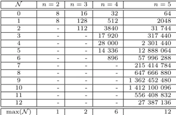
While this is known, we re-checked the distribution of functions with a specific nonlinearity𝒩 for𝑛≤5, confirming the results listed in [10]. Columns for𝑛= 2,3 are not strictly relevant to the following property analysis, but are included for completeness.
𝒩 𝑛= 2 𝑛= 3 𝑛= 4 𝑛= 5
0 8 16 32 64
1 8 128 512 2048
2 - 112 3840 31 744
3 - - 17 920 317 440
4 - - 28 000 2 301 440
5 - - 14 336 12 888 064
6 - - 896 57 996 288
7 - - - 215 414 784
8 - - - 647 666 880
9 - - - 1 362 452 480
10 - - - 1 412 100 096
11 - - - 556 408 832
12 - - - 27 387 136
max(𝒩) 1 2 6 12
Table 4: Distribution of number of𝑓∈ ℬ𝑛with given𝒩-value,𝑛≤5
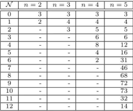
Furthermore, the distribution of the number of orbits within each possible𝒩-
value (i.e., the distribution of nonlinearity of the representatives) is shown in Table 5 – recall that nonlinearity is an affine invariant. Note that there are 16 represen- tatives (and therefore orbits) in 𝑛 = 5 variables where 𝒩 = 5. Further, we can see that there are two orbits with maximum nonlinearity in 𝑛= 4(and therefore two orbits that contain all bent functions in𝑛= 4), and 14 orbits with maximum nonlinearity in𝑛= 5(𝒩 = 6and𝒩 = 12, respectively; recall that the maximum nonlinearity for 𝑛 = 5 is 2𝑛−1−2𝑛−21 = 12, the well known bent concatenation bound).
𝒩 𝑛= 2 𝑛= 3 𝑛= 4 𝑛= 5
0 3 3 3 3
1 2 4 4 4
2 - 3 5 5
3 - - 6 6
4 - - 8 12
5 - - 4 16
6 - - 2 31
7 - - - 46
8 - - - 68
9 - - - 72
10 - - - 73
11 - - - 32
12 - - - 14
Table 5: Distribution of number of orbits with given𝒩-value,𝑛≤5
6. Conclusions
Table 3 summarizes the outcome of our computation to find the number of orbits in each thickness class, for𝑛≤5variables, with the number of orbits and maximum thickness listed. As a double check, the number of equivalence classes (orbits) in ℬ𝑛 matches the one of Harrison [6].
By using the concepts of rigid and representative functions defined in Sections 3 and 4, the thickness distribution of 𝑛 ≤ 5 can be calculated in significantly less time than the time estimation of a brute-force application, by (roughly) 2·106 years. The case of𝑛= 4took little time compared to𝑛= 5(we display in Table 6 the time our computation took; iterations stand for the number of parallel sessions we ran).
Mon. count Functions/Iterations Min. time Max. time Total time (add.)
2 28 / 3 4h 4h 12h
3 134 / 4 6h 12h 1d 12h
4 625 / 4 1d 3h 1d 7h 4d 21h
5 2674 / 8 4d 10h 5d 5h 38d 14h
6 10 195 / 14 1d 14h 3d 19h 39d 17h
7 34 230 / 15 1d 4h 3d 15h 36d 16h
8 100 577 / 20 24s 5d 1h 11d 20h
Total 19d 15h 131d 16h
Table 6: Execution time of the iterations completed by our program
We display in Appendices A and B, the distribution of various cryptographic properties (bentness and semi-bentness, balancedness, etc.) as they relate to thick- ness, for 𝑛 = 4, respectively, 𝑛 = 5. Three physical computers were used for these computations (which took about 35 days): 1) a dedicated Windows server with Intel(R) Xeon(R) E5-2690 v2 3.00 GHz CPU, 20 cores, and 128 GiB RAM, responsible for the bulk of the calculations, 2) a desktop running Ubuntu with Intel(R) Core(TM) i7-6800K 3.40 GHz CPU, 8 cores, and 32 GiB RAM, and fi- nally 3) a desktop running Windows 10 with Intel(R) Core(TM) i5-4460 3.20 GHz CPU, 4 cores, and 16 GiB RAM. The program iterations referenced in Table 6 were run simultaneously and each program was continually updated whenever new representatives were found.
Acknowledgements. The authors would like to thank the referee for the com- ments and the editors for the prompt handling of our paper.
References
[1] J. Boyar,M. G. Find:Constructive Relationships Between Algebraic Thickness and Nor- mality, in: In Fundamentals of Computation Theory, LNCS 9210, Springer, Cham, 2015, pp. 106–117,
doi:https://doi.org/10.1007/978-3-319-22177-9_9.
[2] C. Carlet:Boolean Functions, in: van Tilborg H, ed. byJ. S. C. A., Springer, Boston, MA: Encyclopedia of Cryptography and Security, 2011, pp. 162–164,
doi:https://doi.org/10.1007/978-1-4419-5906-5_336.
[3] C. Carlet:On Cryptographic Complexity of Boolean Functions, in: Proc. 6th Conf. Finite Fields With Applications to Coding Theory, Springer, 2002, pp. 53–69,
doi:https://doi.org/10.1007/978-3-642-59435-9_4.
[4] C. Carlet:On the Degree, Nonlinearity, Algebraic Thickness, and Nonnormality of Boolean Functions, With Developments on Symmetric Functions, IEEE Trans. Inf. Theory 50.9 (2004), pp. 2178–2185,
doi:https://doi.org/10.1109/TIT.2004.833361.
[5] T. W. Cusick,P. Stănică:Cryptographic Boolean Functions and Applications (2nd ed.) Elsevier-Academic Press, 2017,
doi:https://doi.org/10.1016/C2016-0-00852-5.
[6] M. A. Harrison:On the classification of Boolean functions by the general linear and affine groups, Journal of the Society for Industrial and Applied Mathematics 12.2 (1964), pp. 285–
299,doi:https://doi.org/10.1137/0112026.
[7] M. Hopp:Thickness Distribution of Boolean Functions in4and5Variables, Master Thesis, Department of Computing, Mathematics and Physics, Western Norway University of Applied Sciences (2020).
[8] F. J. MacWilliams,N. J. A. Sloane:The theory of error correcting codes, Amsterdam:
North-Holland, 1977.
[9] SageMath:Open-Source Mathematical Software System, Last Accessed: 2020-09-10, url:http://www.sagemath.org.
[10] I. Sertkaya,A. Doğanaksoy:On the Affine Equivalence and Nonlinearity Preserving Bijective Mappings ofF2, International Workshop on the Arithmetic of Finite Fields, WAIFI Arithmetic of Finite Fields, (2014), pp. 121–136,
doi:https://doi.org/10.1007/978-3-319-16277-57.
Appendix A: Property distribution in n = 4, sorted by thickness
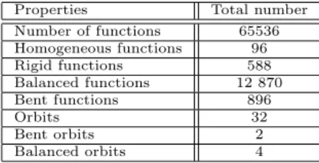
We include here the comparison between various cryptographic properties (homo- geneous, rigid, balanced, bentness, nonlinearity, degree) of Boolean functions as related to thickness for 𝑛= 4variables. Table 7 is a summary of all the property distributions of Tables 8–12 (independent on algebraic thickness).
Properties Total number
Number of functions 65536 Homogeneous functions 96
Rigid functions 588
Balanced functions 12 870
Bent functions 896
Orbits 32
Bent orbits 2
Balanced orbits 4
Table 7: Summary of the property distribution ofn= 4
Properties Nonlinearity Degrees
Number of functions 307 0 31 0 1
Homogeneous functions 52 1 16 1 30
Rigid functions 16 2 120 2 140
Balanced functions 30 3 0 3 120
Bent functions 0 4 140 4 16
Orbits 5 5 0
Bent orbits 0 6 0
Balanced orbits 1
Table 8: Property distribution of functions inℬ4with𝒯4= 1
Properties Nonlinearity Degrees
Number of functions 6804 0 0 0 0
Homogeneous functions 42 1 256 1 0
Rigid functions 64 2 2880 2 1428
Balanced functions 2760 3 560 3 4560
Bent functions 448 4 2660 4 816
Orbits 10 5 0
Bent orbits 1 6 448
Balanced orbits 2
Table 9: Property distribution of functions inℬ4with𝒯4= 2
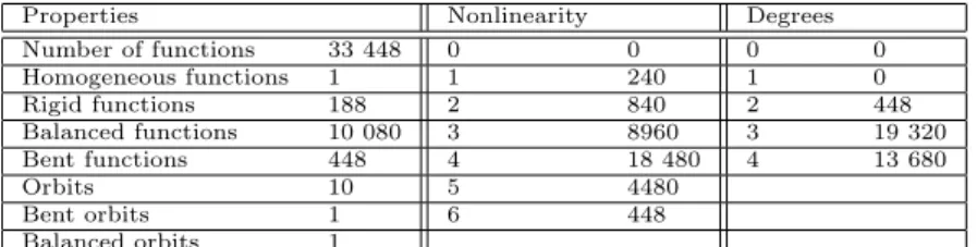
Properties Nonlinearity Degrees
Number of functions 33 448 0 0 0 0
Homogeneous functions 1 1 240 1 0
Rigid functions 188 2 840 2 448
Balanced functions 10 080 3 8960 3 19 320
Bent functions 448 4 18 480 4 13 680
Orbits 10 5 4480
Bent orbits 1 6 448
Balanced orbits 1
Table 10: Property distribution of functions inℬ4with𝒯4= 3
Properties Nonlinearity Degrees
Number of functions 22 288 0 0 0 0
Homogeneous functions 0 1 0 1 0
Rigid functions 271 2 0 2 0
Balanced functions 0 3 8400 3 6720
Bent functions 0 4 6720 4 15 568
Orbits 5 5 7168
Bent orbits 0 6 0
Balanced orbits 0
Table 11: Property distribution of functions inℬ4with𝒯4= 4
Properties Nonlinearity Degrees
Number of functions 2688 0 0 0 0
Homogeneous functions 0 1 0 1 0
Rigid functions 48 2 0 2 0
Balanced functions 0 3 0 3 0
Bent functions 0 4 0 4 2688
Orbits 1 5 2688
Bent orbits 0 6 0
Balanced orbits 0
Table 12: Property distribution of functions inℬ4with𝒯4= 5
Appendix B: Property distribution in n = 5, sorted by thickness
The cryptographic properties dealt with and the goals of the comparison for𝑛= 5 are the same as for 𝑛= 4.
Properties Total amount
Number of functions 4 294 967 296 Homogeneous functions 2111
Rigid functions 211 259
Balanced functions 601 080 390 Semi-Bent functions 14 054 656
Number of orbits 382
Semi-Bent orbits 9
Balanced orbits 38
Table 13: Summary of the property distribution ofn = 5
Properties Nonlinearity Degrees
Number of𝑓 2451 0 63 0 1
Homogeneous𝑓 203 1 32 1 62
Rigid𝑓 32 2 496 2 620
Balanced𝑓 62 3 0 3 1240
Semi-Bent𝑓 0 4 1240 4 496
Orbits 6 5 0 5 32
Semi-Bent orbits 0 6 0
Balanced orbits 1 7 0
8 620
9 0
10 0
11 0
12 0
Table 14: Property distribution of functions inℬ5with𝒯5= 1
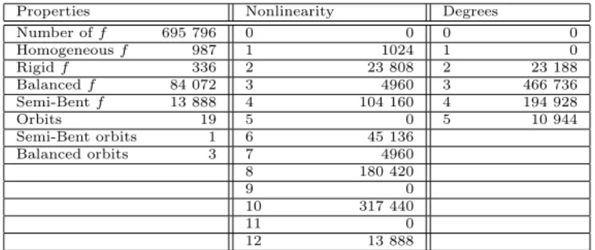
Properties Nonlinearity Degrees
Number of𝑓 695 796 0 0 0 0
Homogeneous𝑓 987 1 1024 1 0
Rigid𝑓 336 2 23 808 2 23 188
Balanced𝑓 84 072 3 4960 3 466 736
Semi-Bent𝑓 13 888 4 104 160 4 194 928
Orbits 19 5 0 5 10 944
Semi-Bent orbits 1 6 45 136
Balanced orbits 3 7 4960
8 180 420
9 0
10 317 440
11 0
12 13 888
Table 15: Property distribution of functions inℬ5with𝒯5= 2
Properties Nonlinearity Degrees
Number of𝑓 31 424 328 0 0 0 0
Homogeneous𝑓 859 1 992 1 0
Rigid𝑓 2480 2 7440 2 41 664
Balanced𝑓 4 228 896 3 158 720 3 7620792
Semi-Bent𝑓 874 944 4 1 536 360 4 22 119 120
Orbits 46 5 34 720 5 1 642 752
Semi-Bent orbits 3 6 2 138 752
Balanced orbits 6 7 853 120
8 15 323 920
9 317 440
10 9 900 160
11 277 760
12 874 944
Table 16: Property distribution of functions inℬ5with𝒯5= 3
Properties Nonlinearity Degrees
Number of𝑓 240 101 200 0 0 0 0
Homogeneous𝑓 61 1 0 1 0
Rigid𝑓 11 520 2 0 2 0
Balanced𝑓 15 582 336 3 153 760 3 23 290 176
Semi-Bent𝑓 2 499 840 4 659 680 4 168 597 840
Orbits 81 5 1 416 576 5 48 213 184
Semi-Bent orbits 2 6 10 731 952
Balanced orbits 6 7 17 541 536
8 112 334 080
9 18 213 120
10 63 162 624
11 10 888 192
12 4 999 680
Table 17: Property distribution of functions inℬ5with𝒯5= 4
Properties Nonlinearity Degrees
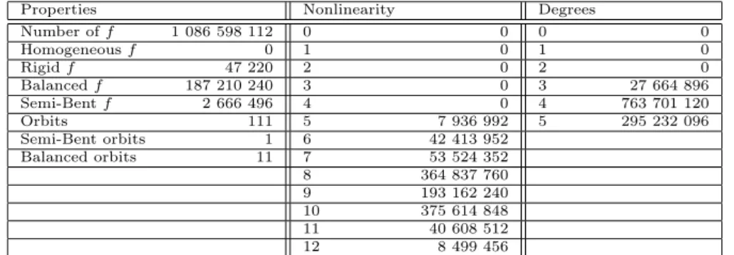
Number of𝑓 1 086 598 112 0 0 0 0
Homogeneous𝑓 0 1 0 1 0
Rigid𝑓 47 220 2 0 2 0
Balanced𝑓 187 210 240 3 0 3 27 664 896
Semi-Bent𝑓 2 666 496 4 0 4 763 701 120
Orbits 111 5 7 936 992 5 295 232 096
Semi-Bent orbits 1 6 42 413 952
Balanced orbits 11 7 53 524 352
8 364 837 760
9 193 162 240
10 375 614 848
11 40 608 512
12 8 499 456
Table 18: Property distribution of functions inℬ5with𝒯5= 5
Properties Nonlinearity Degrees
Number of𝑓 1 842 215 424 0 0 0 0
Homogeneous𝑓 0 1 0 1 0
Rigid𝑓 59 760 2 0 2 0
Balanced𝑓 308 646 912 3 0 3 7 999 488
Semi-Bent𝑓 7 999 488 4 0 4 951 105 792
Orbits 81 5 3 499 776 5 883 110 144
Semi-Bent orbits 2 6 2 666 496
Balanced orbits 9 7 96 827 136
8 154 990 080
9 694 122 240
10 788 449 536
11 88 660 992
12 12 999 168
Table 19: Property distribution of functions inℬ5with𝒯5= 6
![Table 2: Number of affine equivalence classes of Boolean functions [6]](https://thumb-eu.123doks.com/thumbv2/9dokorg/790062.36935/11.722.253.470.114.226/table-number-affine-equivalence-classes-boolean-functions.webp)