Use of Multi-parametric Quadratic Programming in Fuzzy Control Systems

Use of Multi-parametric Quadratic

Programming in Fuzzy Control Systems

Zsuzsa Preitl, Radu-Emil Precup

Dept. of Automation and Applied Inf., “Politehnica” University of Timisoara Bd. V. Parvan 2, RO-300223 Timisoara, Romania

E-mail: zsuzsa.preitl@aut.upt.ro, radu.precup@aut.upt.ro

József K. Tar, Márta Takács

Institute of Intelligent Engineering Systems, Budapest Tech Bécsi út 96/B, H-1034 Budapest, Hungary

E-mail: tar.jozsef@nik.bmf.hu, takacs.marta@nik.bmf.hu

Abstract: The paper presents some main aspects regarding multi-parametric quadratic programming (mp-QP) problems. Model Predictive Control (MPC) is considered as a particular mp-QP problem, and this powerful tool is applied for control and simulation through a case study. Since the solutions to mp-QP problems can be expressed as piecewise affine linear functions of the state, a new implementation in terms of adaptive network- based fuzzy inference systems is proposed. The presentation is focused on the double integrator plant as a frequently appearing case study (electrohydraulic servo-system).

Keywords: Multi-parametric quadratic programming, model predictive control, adaptive network-based fuzzy inference systems, Multi-Parametric Toolbox

1 Introduction

By multi-parametric programming, a linear or quadratic optimization problem is solved off-line. The multi-parametric approaches are based on off-line computation of the feedback law, having their advantages and disadvantages [15].

The resulting explicit controller generates regions for the control law, their number increases with the complexity of the problem, being able to become easily prohibitive. This is mainly due to the exponential number of transitions between regions, which can occur when a controller is developed in a dynamic programming fashion.

The main method to solve multi-parametric linear programming problems was proposed in [1] and described in [2]. The method is based on constructing the critical regions iteratively, by examining the graph of bases associated to the linear programming tableau of the original problem. Other methods are presented in [3, 4, 5].

The most cited method to solve multi-parametric quadratic programming (mp-QP) problems was formulated in [6]. The method constructs a critical region in a vicinity of a given parameter using Karush-Kuhn-Tucker conditions for optimality, and then it explores recursively the parameter space outside such regions. A very efficient implementation until now is given in [2], and other methods to solve mp-QP problems are presented in [7, 8, 9].

Model predictive control (MPC) represents the accepted standard for complex constrained control problems in industrial applications [10]. During each sampling interval, starting at the current state, an open-loop optimal control problem is solved over a finite horizon, leading to a moving horizon strategy. The drawback of MPC is the relatively high on-line computational effort, which limits its applicability to control relatively slow plants.

This paper addresses the process of moving the necessary calculations for the implementation of MPC off-line in the conditions of considering it a special case of mp-QP problem [6]. In case of MPC algorithms solved in terms of mp-QP problems with piecewise affine linear solutions as functions of the state, the implementation problem is relatively complex [10].

One of the aims of the paper is to propose a new implementation of mp-QP solutions in terms of adaptive network-based fuzzy inference systems [13, 14].

This paper is organized as follows. The next Section presents the main aspects concerning the problem setting in mp-QP and an algorithm to solve mp-QP problems accompanied by comments. In Section 3 the MPC as particular case of mp-QP is analyzed. Then Section 4 is dedicated to the implementation of the piecewise affine linear solutions as functions of the state in case of mp-QP in terms of a neuro-fuzzy approach using adaptive network-based fuzzy inference systems. Section 5 deals with the applications of the mp-QP problems in case studies concentrated on the well accepted double integrator plant in several settings, and the last Section highlights the conclusions.

2 Problem Setting in Multi-parametric Quadratic Programming

The definition of an mp-QP problem is given in terms of [2, 6]:

x S W z G

Hz ' 2 z ) 1 x , z ( minJ ) x (

Jˆ subjectto

z

+

≤

=

= ^{, (1)}

where z∈R^s are the optimization (manipulated) variables, x∈Rⁿ is the parameter vector, H∈R^s×s, H >0, W∈R^m, S∈R^m×n. Other non- homogenous problems with the general objective function (2):

Fz x Hz z x z

J( , )= ' + ' , (2)

can always be transformed in the problem (1) using the variable substitution (3):

x F H z

z '

~= + −1 . (3)

To solve the mp-QP problem (1) it is necessary to calculate the polyhedral partition of the parameter space. With this respect, the following three definitions are useful [15].

Definition 1: A convex set Q⊆Rⁿ given as an intersection of a finite number of closed half-spaces:

{

}

= |

Q , (4)

is called polyhedron.

Definition 2: A bounded polyhedron P⊆Rⁿ:

{

}

= |

P , (5)

is called polytope.

It is obvious from these two definitions that every polytope represents a convex, compact (i.e., bounded and closed) set.

Definition 3: The linear inequality a'x≤b is called valid for a polyhedron P if b

x

a' ≤ holds for all x∈P. A subset of a polyhedron is called a face of P if it is represented as:

{

}

∩

=P | '

F , (6)

for some valid inequality a'x≤b. The faces of polyhedron P of dimension 0, 1, (n – 2) and (n – 1) are called vertices, edges, ridges and facets, respectively.

Connecting to the mp-QP problem (1), given a close polyhedral set K⊂Rⁿ of parameters:

{

}

= |

K , (7)

it is denoted by Kˆ⊂K the region of parameters x∈K such that the mp-QP problem (1) is feasible and the optimum Jˆ(x) is finite.

The fundamental aspect of multi-parametric approaches to optimization is that for any given x∈K, Jˆ(x) denotes the minimum value of the objective function in (1) for x=x, the function Jˆ:Kˆ→R called value function, expresses the dependence on x of the minimum value of the objective function over Kˆ, and the single-valued function zˆ:Kˆ→R describes for any fixed x∈Kˆ the optimizer

) ˆ(x

z corresponding to Jˆ(x).

To solve the mp-QP problem (1), the algorithm consisting of the following steps can be used [2]:

- Define the matrices H, G, W and S of the problem and set K in (7) according to the desired CS performance objectives.

- Calculate the partition of K according to the steps 1 … 9:

1: Let x₀∈K the centre of the largest ball contained in K for which a feasible z exists, and ε the solution to the linear programming problem (8) related to this centre:

W Sx Gz n i Z T f x T

f _{i i i T}

x z

≤

−

=

≤ +

=

ε

max

,

, (8) where nT stands for the number of rows Ti of the matrix T.

2: If ε ≤ 0, then the partition is calculated (no full dimensional critical region is in K). Else, continue with step 3.

3: Solve the mp-QP (1) for x = x0 to obtain (zˆ₀,λˆ₀).

4: Determine the set of active constraints A0 when z=zˆ₀, x = x0, and build GA0, WA0 and SA0.

5: If r = rank GA0 < l (the number of rows of GA0), then take a subset of r linearly independent rows, and redefine GA0, WA0 and SA0 accordingly.

6: Determine ˆ ( )

0 x

λ A and zˆ_A0(x) from (9):

) ˆ ( ' )

ˆ ( ), (

) ' (

) ˆ (

0 1 0

0 0 1 0

1 0 0

0 x G_A H G_A W_A S_A x z_A x H G_{A A} x

A = − + = − λ

λ ^{− − −} . (9)

7: Characterize the critical region from (10) where the first inequality corresponds to the constraints in (1) and the second one to the Lagrange multipliers in (9) that must remain nonnegative as x is variable:

. 0 ) (

) ' (

, )

( ) ' (

'

0 1 0

1 0 0

0 1 0

1 0 0 1 0

≥ +

−

+

≤ +

−

−

−

−

−

x S W

G H G

Sx W x S W

G H G G GH

A A

A A

A A

A A

A (10)

8: Define and partition the rest of the region according to [2].

9: Partition each new sub-region.

This algorithm explores the set K of parameters recursively. The partition of the rest of the region into polyhedral sets can be represented as a search tree, with a maximum depth equal to the number of combinations of active constraints.

Concerning the controller implementation, at each sampling interval a polyhedral partition is calculated, with as many different partitions as the length of the prediction horizon. If the Receding Horizon Technique (RHT) is used, then only one polyhedral partition is used out of those which were calculated. That is the reason why the generated controller has only one form. Concerning the algorithm presented before, the following three comments must be highlighted.

Firstly, the very first partition is based on choosing x0 adequately. Since a choice is involved, there is no single solution to the algorithm.

Secondly, the determination of the set of active constraints is critical, since the remaining regions are partitioned based on some combination of active constraints. Namely, each region represents a region in the parameter space where a number of combinations is active. There is an upper bound for the maximum number, 2^m, where m is the cardinal of the set of all constraints.

Thirdly, the selection of active constraints is not a simple task. All algorithms are based on an iterative procedure that builds up the parametric solution by generating new polyhedral regions of the parameter space at each step. The methods differ in the way they explore the parameter space, that is, in the way they identify active constraints corresponding to the critical regions neighbouring to a given critical region [2]. In [6] the unconstrained critical region is constructed and then the neighbouring critical regions are generated by enumerating all possible combinations of active constraints.

Note that the expression of (9) and the fact that the algorithm is applied for several regions, the control signal will be a piecewise affine linear function of the state.

3 Model Predictive Control as Multi-parametric Quadratic Programming Problem

MPC is employed to solve the constrained regulation problem [6] consisting of regulating towards the origin the plant represented by the discrete-time linear time invariant model (11):

), ( ) (

), ( ) ( ) 1 (

t x C t y

t u B t x A t

x

=

+

=

+ (11)

fulfilling the constraints (12):

max min

max

min y(t) y , u u(t) u

y ≤ ≤ ≤ ≤ , (12)

at all time instants t ≥ 0, where x(t) ∈ Rⁿ, u(t) ∈ R^m and y(t) ∈ R^p are the state, input and output vectors, respectively, the variables in (12) are vectors with appropriate dimensions and the pair (A, B) is stabilizable.

Assuming that the state x(t) is fully available at the current time instant t, the MPC is defined in terms of (13):

.

, , 0 ,

, 0 , ),

(

, , 0 ,

, , 1 ,

subject to

] '

' [

' )) ( , ( ]'

ˆ' ,..., ˆ' ˆ [

|

|

|

|

| 1

|

max min

max

| min

1

0 | |

|

| ]'

' ,..., ' [ 1

1

arg min

1 1

y u

t k t k t

t k t t k t

k t t k t t k t

k t

c k

t

c t

k t

Ny

k

k t k t t k t t k t

t Ny t t Ny t u

u U Nu t

N k N x K u

k x C y

k u B x A x

t x x

N k u u u

N k y y y

u R u Qx x

Px x

t x U J u

u U

Nu t

<

≤

=

≥

=

≥ +

=

=

=

≤

≤

=

≤

≤

+ +

+

=

=

=

+ +

+ +

+ +

+ +

+ +

−

= + + + +

+ +

=

− +

∑

− +

(13)

The MPC problem (13) is solved at each time instant t, where x_t+k|t is referred to as the predicted state vector at time t+k, obtained by applying the input sequence ut, …, ut+k−1 to the plant (11) starting from the state x(t) in the conditions of K being the state-feedback gain. It is assumed in (13) that Q=Q' ≥0, R=R' >0,

≥0

P and (Q=C' C,A) is detectable. The other parameters in (13) specific to MPC are Ny, Nu and Nc representing the output, input and constraint horizon, respectively, with Nu ≤ Ny and Nc ≤ Ny – 1. Substituting the state vector x_t+k|t:

∑

= + −−

+ = + ¹

0 1

| x(t) ^k

j

j k t j k

t k

t A A Bu

x , (14)

(13) can be re-expressed as the mp-QP problem (15):

), (

subject to )

( ' 2 '

) 1 ( ) ( 2 ' )) 1 (

(

min

t Ex W GU

U F t x U H U t

Yx t x t x V

U

+

≤

+ +

= (15)

where the column vector U ∈ R^s, s = mNu, is the optimization vector, H =H' >0, and the matrices H, F, Y, G, W and E are obtained from Q, R and (13) [6].

Connecting the approaches in Section 2 and Section 3, the control signal elaborated by the model predictive controller is also a piecewise affine linear function of the state. The following Section will be dedicated to a neuro-fuzzy implementation of the controllers as solutions to mp-QP problems.

4 Neuro-fuzzy Implementation of Piecewise Affine Linear Functions of the State

Examining the algorithm presented in Section 2, the control signal u as piecewise affine linear function is considered in the particular case of a second-order system, n = 2, where the general function can be expressed as:

) , (x₁ x₂ f

u= . (16)

Considering three linguistic terms for each of the two input variables, defined in their initial forms in Fig. 1, the complete rule base of a Takagi-Sugeno fuzzy system [16] consisting of 9 rules, R1 … R9, can be expressed in terms of (17):

] [

THEN ] IS [ ] IS [ IF :

] [

THEN ] IS [ ] IS [ IF :

] [

THEN ] IS [ ] IS [ IF :

] [

THEN ] IS [ ] IS [ IF :

] [

THEN ] IS [ ] IS [ IF :

] [

THEN ] IS [ ] IS [ IF :

] [

THEN ] IS [ ] IS [ IF :

] [

THEN ] IS [ ] IS [ IF :

] [

THEN ] IS [ ] IS [ IF :

9 2 9 1 9 2

2 1

1 9

8 2 8 1 8 2

2 1

1 8

7 2 7 1 7 2

2 1

1 7

6 2 6 1 6 2

2 1

1 6

5 2 5 1 5 2

2 1

1 5

4 2 4 1 4 2

2 1

1 4

3 2 3 1 3 2

2 1

1 3

2 2 2 1 2 2

2 1

1 2

1 2 1 1 1 2

2 1

1 1

C x B x A u X

x AND X

x R

C x B x A u X

x AND X

x R

C x B x A u X

x AND X

x R

C x B x A u X

x AND X

x R

C x B x A u X

x AND X

x R

C x B x A u X

x AND X

x R

C x B x A u X

x AND X

x R

C x B x A u X

x AND X

x R

C x B x A u X

x AND X

x R

P P

P Z

P N

Z P

Z Z

Z N

N P

N Z

N N

+ +

=

+ +

=

+ +

=

+ +

=

+ +

=

+ +

=

+ +

=

+ +

=

+ +

=

. (17)

The membership function shapes in Fig. 1 have been obtained supposing that the fuzzy system includes the scaling factors (which can be non-linear in case of implementing MPC), and they correspond to so-called dsigmoidal-type functions according to [14] with the expressions in (18) as difference of two sigmoidal ones:

}.

11 , 9 , 7 , 5 , 3 , 1 { }, , {

)]}, (

exp{

1 /{

1 )]}

( exp{

1 /{

1 ) (

2 1

1 1

∈

∈

−

− +

−

−

− +

= _{+ +}

i x x x

c x a c

x a

x _{i i i i}

μi ₍₁₈₎

In the conditions of using use the max and min operators in the inference engine and the weighted average method for defuzzification due to the special form of the consequence in each rule it is easy to observe that the Takagi-Sugeno fuzzy system described here is well suited to model piecewise affine linear functions of the state appearing in case of mp-QP problems.

Figure 1

Initial membership functions of input linguistic terms

The adaptive network-based fuzzy inference system, with the schematic diagram illustrated in Fig. 2, has 5 layers:

- Layer I: The inputs x1 and x2 are passed through the input linguistic terms with the membership functions having the parameters presented in (18), - Layer II: The fuzzy rules in (17) are constructed according to the inference

engine using the product (П) of the two antecedents, the output of each node representing the firing strength of a rule,

- Layer III: The firing strengths are normalized dividing them to the sum of all rule firing strengths,

- Layer IV: The normalized firing strength is multiplied by the output functions of the fuzzy inference system,

- Layer V: The overall system output is calculated as the sum of all incoming signals.

Due to this structure similar to that of certain neural networks, the learning techniques specific to neural networks can be applied to minimize the quadratic objective function E:

∑

−

= ^N

i

i d

i u

u E

1

)2

( , (19)

where: uid – desired control signal, piecewise affine linear function of the state, to be implemented by the Takagi-Sugeno fuzzy system, ui – control signal elaborated by the Takagi-Sugeno fuzzy system, N – number of input-output data pairs.

Figure 2

Schematic diagram of adaptive network-based fuzzy inference system

Minimizing the objective function in (19) using the adaptive structure presented in Fig. 2 and appropriate learning techniques leads to the correction of the parameters of the Takagi-Sugeno fuzzy systems in both the antecedents and the consequents.

5 Case Study

A powerful calculation and simulation tool for multiparametric programming consists in the Multi-Parametric Toolbox (MPT). In the paper the MPT is used for modelling, control and simulation of a double integrator plant [17] in its continuous-time representation (for zero initial conditions) (20):

) 1 ( )

( ₂u s s s

y = , (20)

its equivalent discrete-time state-space representation obtained discretizing in terms of the forward rectangular method for a sampling period of 1 sec., is:

[ ]

(

), 1 ( ) 0 1 ( 0

1 ) 1 1 (

t x t

y

t u t x t

x

=

⎥⎦

⎢ ⎤

⎣ +⎡

⎥⎦

⎢ ⎤

⎣

=⎡

+ (21)

and the system constraints are:

15 15

15 15

1

1≤ ≤ − ≤ ≤ − ≤ _{1 2}≤

− u , y , x,x . (22)

The objective is to regulate the double integrator (21) towards the origin while minimizing the following quadratic performance index and input constraint [6]:

1 1 , )]

( 01 . 0 ) ( ) ( ' [

0

2 − ≤ ≤

+

=

∑

=

u t

u t

y t y J

t

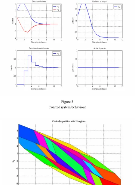
. (24) This problem can be solved by using the MPC algorithm in (13) with Nu = Ny = 2,

R = 0.01, Q11 = 1, Q12 = Q21 = Q22 = 0, and the matrices K and P obtained solving a Riccati equation [6]. The CS behaviour for initial conditions of (21) is illustrated in Fig. 3.

Applying the mp-QP algorithm presented in Section 2 leads in the first phase to 25 controller regions. Merging the controller regions, in this case it was achieved from 25 regions to 21 regions, for the last sampling interval. These regions can be plotted as in Figure 4.

Applying the mp-QP algorithm the control signal will have the piecewise affine linear form (23) that can be well modelled using the neuro-fuzzy approach presented in the previous Section.

Figure 3 Control system behaviour

Figure 4 Controller regions

⎥⎥

⎥⎥

⎥⎥

⎥⎥

⎥⎥

⎥⎥

⎥⎥

⎥⎥

⎥⎥

⎥⎥

⎥⎥

⎥⎥

⎥⎥

⎥⎥

⎥⎥

⎥

⎦

⎤

⎢⎢

⎢⎢

⎢⎢

⎢⎢

⎢⎢

⎢⎢

⎢⎢

⎢⎢

⎢⎢

⎢⎢

⎢⎢

⎢⎢

⎢⎢

⎢⎢

⎢⎢

⎢

⎣

⎡

+

⎥⎥

⎥⎥

⎥⎥

⎥⎥

⎥⎥

⎥⎥

⎥⎥

⎥⎥

⎥⎥

⎥⎥

⎥⎥

⎥⎥

⎥⎥

⎥⎥

⎥⎥

⎥

⎦

⎤

⎢⎢

⎢⎢

⎢⎢

⎢⎢

⎢⎢

⎢⎢

⎢⎢

⎢⎢

⎢⎢

⎢⎢

⎢⎢

⎢⎢

⎢⎢

⎢⎢

⎢⎢

⎢

⎣

⎡

=

760682 1.72724809 -

760682 1.72724809

751597 0.87990997 -

751597 0.87990997

000000 1.00000000

000000 1.00000000

000000 1.00000000

000000 1.00000000

000000 1.00000000

000000 1.00000000

000000 1.00000000

792517 0.45607670 -

792517 0.45607670

000000 1.00000000 -

000000 1.00000000 -

000000 1.00000000 -

000000 1.00000000 -

000000 1.00000000 -

000000 1.00000000 -

000000 1.00000000 -

0

842852 1.21419288 -

842852 0.21419288 -

842852 1.21419288 -

842852 0.21419288 -

358994 1.33799618 -

245851 0.34224024 -

358994 1.33799618 -

245851 0.34224024 -

0 0

0 0

0 0

0 0

0 0

0 0

0 0

747608 1.42514751 -

869264 0.43504549 -

747608 1.42514751 -

869264 0.43504549 -

0 0

0 0

0 0

0 0

0 0

0 0

0 0

132617 1.54562698 -

112176 0.57917087 -

x u

.(23)

The control law can also be plotted, as presented in Fig. 5.

Figure 5

Control signal over the regions

Closed loop trajectories in the state-space can be plotted as well, for all initial conditions that are feasible. For this problem setting (regulation towards origin) for several initial conditions these trajectories are depicted in Fig. 6.

Figure 6

Closed loop trajectories for different initial conditions

Transforming the MPC problem (13) into a mp-QP one (15), the solution to the MPC algorithm can be calculated as piecewise affine linear functions of the state.

Conclusions

The paper presents aspects concerning the mp-QP problems with solutions implemented in state-feedback form as piecewise affine linear functions of the state. These solutions are subject to very convenient implementations as Takagi- Sugeno fuzzy systems using neuro-fuzzy techniques. An example of a double integrator plant is presented, applying the so-called MPT toolbox.

Future research will deal with the computer-aided solution of mp-QP and MPC problems. On the other hand, applications to discrete-event systems in manufacturing and robot control will be tackled [18, 19, 20].

Acknowledgement

The support stemming from the cooperation between Budapest Tech Polytechnical Institution and “Politehnica” University of Timisoara in the framework of the Hungarian-Romanian Intergovernmental Science & Technology Cooperation Program no. 35 ID 17 and from two CNCSIS grants is kindly acknowledged.

References

[1] T. Gal, J. Nedoma: Multiparametric Linear Programming, in Management Science, Vol. 18, 1972, pp. 406-442

[2] F. Borelli: Constrained Optimal Control of Linear and Hybrid Systems, Springer-Verlag, Berlin, Heidelberg, 2003

[3] M. Schechter: Polyhedral Functions and Multiparametric Linear Programming, in Journal of Optimal Theory and Applications, Vol. 53, No.

2, 1987, pp. 269-280

[4] T. Gal: Postoptimal Analyses, Parametric Programming, and Related Topics, de Gruyer, Berlin, 2^nd edition, 1995

[5] C. Filippi: On the Geometry of Optimal Partition Sets in Multiparametric Linear Programming, Technical Report 12, Department of Pure and Applied Mathematics, University of Padova, Italy, 1997

[6] A. Bemporad, M. Morari, V. Dua, S. Pistikopoulos: The Explicit Linear Quadratic Regulator for Constrained Systems, in Automatica, Vol. 38, No.

1, 2002, pp. 3-20

[7] M. M. Seron, J. A. De Doná, G. C. Goodwin: Global Analytical Model Predictive Control with Input Constraints, in Proceedings of 39^th IEEE Conference on Decision and Control, Sydney, Australia, 2000, pp. 154-159 [8] P. Tøndel, T. A. Johansen, A. Bemporad: An Algorithm for Multi- Parametric Quadratic Programming and Explicit MPC Solutions, in Proceedings of 40^th IEEE Conference on Decision and Control, Orlando, FL, Vol. 3, 2001, pp. 2849-2854

[9] M. Baotic: An Efficient Algorithm for Multi-Parametric Quadratic Programming, Technical Report AUT02-04, Automatic Control Laboratory, ETH Zürich, Switzerland, 2002

[10] E. F. Camacho, C. Bordons: Model Predictive Control, Springer-Verlag, Berlin, Heidelberg, 2^nd edition, 2004

[11] H. W. Chiou, E. Zafiriou: Frequency Domain Design of Robustly Stable Constrained Model Predictive Controllers, in Proceedings of the American Control Conference, Baltimore, USA, Vol. 3, 1994, pp. 2852-2856

[12] T. A. Johansen, I. Petersen, O. Slupphaug: On Explicit Suboptimal LQR with State and Input Constraints, in Proceedings of 39^th IEEE Conference on Decision and Control, Sydney, Australia, 2000, pp. 662-667

[13] J. Jang: ANFIS: Adaptive Network-based Fuzzy Inference System, in IEEE Transactions on Systems, Man, and Cybernetics, Vol. 23, No. 3, 1993, pp.

665-685

[14] Mathworks: Fuzzy Logic Toolbox User’s Guide V. 3, Natick, MA, 2000

[15] M. Kvasnica, P. Grieder, M. Baotić, F. J. Christophersen: Multi-Parametric Toolbox (MPT), Tutorial

[16] T. Takagi, M. Sugeno: Fuzzy Identification of Systems and its Applications to Modelling and Control, in IEEE Transactions on Systems, Man, and Cybernetics, Vol. 15, No. 1, 1985, pp. 116-132

[17] S. Preitl, R-E. Precup, Zsuzsa Preitl: Sensitivity Analysis of Low Cost Fuzzy Controlled Servo Systems, 16^th World Congress of International Federation of Automatic Control 2005, Prague, Czech Republic, Preprints, Editors: P. Horacek, M. Simandl, P. Zitek, DVD, paper index 1794 (6 pages)

[18] L. Horváth, I. J. Rudas: Modeling and Problem Solving Methods for Engineers, Elsevier, Academic Press, 2004

[19] L. Horváth, I. J. Rudas, C. Couto: Integration of Human Intent Model Descriptions in Product Models, in Digital Enterprise - New Challenges Life-Cycle Approach in Management and Production, Kluwer Academic Publishers, 2001, pp. 1-12

[20] L. Horváth, I. J. Rudas, J. F. Bitó, A. Szakál: Adaptive Model Objects for Robot Related Applications of Product Models, in Proc. 2004 IEEE International Conference on Robotics & Automation ICRA 2004, New Orleans, LA, USA, 2004, pp. 3137-3142