Physics II.
Gy¨ orgy H´ ars
G´ abor Dobos
2013.04.30
Contents
1 Electrostatic phenomena - Gy¨orgy H´ars 3
1.1 Fundamental experimental phenomena . . . 3
1.2 The electric field . . . 4
1.3 The flux . . . 5
1.4 Gauss’s law . . . 6
1.5 Point charges and the Coulomb’s law . . . 7
1.6 Conservative force field . . . 8
1.7 Voltage and potential . . . 9
1.8 Gradient . . . 10
1.9 Spherical structures . . . 11
1.9.1 Metal sphere . . . 11
1.9.2 Sphere with uniform space charge density . . . 13
1.10 Cylindrical structures . . . 15
1.10.1 Infinite metal cylinder . . . 15
1.10.2 Infinite cylinder with uniform space charge density . . . 17
1.11 Infinite parallel plate with uniform surface charge density . . . 20
1.12 Capacitors . . . 21
1.12.1 Cylindrical capacitor . . . 22
1.12.2 Spherical capacitor . . . 24
1.13 Principle of superposition . . . 25
2 Dielectric materials - Gy¨orgy H´ars 27 2.1 The electric dipole . . . 27
2.2 Polarization . . . 28
2.3 Dielectric displacement . . . 30
2.4 Electric permittivity (dielectric constant) . . . 32
2.5 Gauss’s law and the dielectric material . . . 32
2.6 Inhomogeneous dielectric materials . . . 33
2.7 Demonstration examples . . . 35
2.7.1 . . . 35
2.7.2 . . . 39
2.8 Energy relations . . . 39
2.8.1 Energy stored in the capacitor . . . 39
2.8.2 Principle of the virtual work . . . 42
3 Stationary electric current (direct current) - Gy¨orgy H´ars 44 3.1 Definition of Ampere . . . 44
3.2 Current density (j) . . . 45
3.3 Ohm’s law . . . 46
3.4 Joule’s law . . . 47
3.5 Microphysical interpretation . . . 47
4 Magnetic phenomena in space - Gy¨orgy H´ars 49 4.1 The vector of magnetic induction (B) . . . 49
4.2 The Lorentz force . . . 50
4.2.1 Cyclotron frequency . . . 51
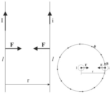
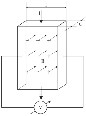
4.2.2 The Hall effect . . . 53
4.3 Magnetic dipole . . . 54
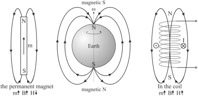
4.4 Earth as a magnetic dipole . . . 57
4.5 Biot-Savart law . . . 58
4.5.1 Magnetic field of the straight current . . . 59
4.5.2 Central magnetic field of the polygon and of the circle . . . 60
4.6 Ampere’s law . . . 61
4.6.1 Thick rod with uniform current density . . . 63
4.6.2 Solenoid . . . 64
4.6.3 Toroidal coil . . . 65
4.7 Magnetic flux . . . 66
5 Magnetic field and the materials - Gy¨orgy H´ars 67 5.1 Three basic types of magnetic behavior . . . 67
5.2 Solenoid coil with iron core . . . 69
5.3 Ampere’s law and the magnetic material . . . 71
5.4 Inhomogeneous magnetic material . . . 72
5.5 Demonstration example . . . 75
5.6 Solenoid with iron core . . . 77
6 Time dependent electromagnetic field - Gy¨orgy H´ars 80 6.1 Motion related electromagnetic induction . . . 80
6.1.1 Plane generator (DC voltage) . . . 80
6.1.2 Rotating frame generator (AC voltage) . . . 83
6.1.3 Eddy currents . . . 84
6.2 Electromagnetic induction at rest . . . 86
2
6.2.1 The mutual and the self induction . . . 86
6.2.2 Induced voltage of a current loop . . . 87
6.2.3 The transformer . . . 88
6.2.4 Energy stored in the coil . . . 93
6.3 The Maxwell equations . . . 94
7 Electromagnetic oscillations and waves - G´abor Dobos 96 7.1 Electrical oscillators. . . 96
7.2 Electromagnetic waves in perfect vacuum . . . 99
7.3 Electromagnetic waves in non-conductive media . . . 101
7.4 Direction of the E and B fields . . . 102
7.5 Pointing Vector . . . 102
7.6 Light-pressure . . . 103
7.7 Skin depth . . . 106
7.8 Reflection and refraction . . . 108
8 Geometrical Optics - G´abor Dobos 111 8.1 Total internal reflection . . . 111
8.2 Spherical Mirror . . . 112
8.3 Thin spherical lenses . . . 117
8.4 Projection by spherical lenses and mirrors . . . 120
8.5 Aberrations . . . 123
9 Wave optics - G´abor Dobos 127 9.1 Young’s double slit experiment. . . 127
9.2 Coherence . . . 130
9.3 Multiple slit diffraction . . . 132
9.4 Fraunhofer diffraction. . . 137
9.5 Thin layer interference . . . 142
10 Einstein’s Special Theory of Relativity – G´abor Dobos 148 10.1 The Aether Hypothesis and The Michelson-Morley Experiment. . . 148
10.2 Einstein’s Special Theory of Relativity . . . 152
10.3 Lorentz contraction and time dilatation . . . 155
10.4 Velocity addition . . . 159
10.5 Connection between relativistic and classical physics. . . 160
Introduction
Present work is the summary of the lectures held by the author at Budapest University of Technology and Economics. Long verbal explanations are not involved in the text, only some hints which make the reader to recall the lecture. Refer here the book: Alonso/Finn Fundamental University Physics, Volume II where more details can be found.
Physical quantities are the product of a measuring number and the physical unit.
In contrast to mathematics, the accuracy or in other words the precision is always a secondary parameter of each physical quantity. Accuracy is determined by the number of valuable digits of the measuring number. Because of this 1500 V and 1.5 kV are not equivalent in terms of accuracy. They have 1 V and 100 V absolute errors respectively.
The often used term relative error is the ratio of the absolute error over the nominal value. The smaller is the relative error the higher the accuracy of the measurement.
When making operations with physical quantities, remember that the result may not be more accurate than the worst of the factors involved. For instance, when dividing 3.2165 V with 2.1 A to find the resistance of some conductor, the result 1.5316667 ohm is physically incorrect. Correctly it may contain only two valuable digits, just like the current data, so the correct result is 1.5 ohm.
The physical quantities are classified as fundamental quantities and derived quan- tities. The fundamental quantities and their units are defined by standard or in other words etalon. The etalons are stored in relevant institute in Paris. The fundamental quantities are the length, the time and the mass. The corresponding units are meter (m), second (s) and kilogram (kg) respectively. These three fundamental quantities are sufficient to build up the mechanics. The derived quantities are all other quantities which are the result of some kind of mathematical operations. To describe electric phenomena the fourth fundamental quantity has been introduced. This is ampere (A) the unit of electric current. This will be used extensively in Physics 2, when dealing with electricity.
4
Chapter 1
Electrostatic phenomena - Gy¨ orgy H´ ars
1.1 Fundamental experimental phenomena
Electrostatics deals with the phenomena of electric charges at rest. Electric charges can be generated by rubbing different insulating materials with cloth or fur. The de- vice called electroscope is used to detect and roughly measure the electric charge. By rubbing a glass rod and connecting it to the electroscope the device will indicate that charge has been transferred to it. By doing so second time the electroscope will indicate even more charges. Accordingly the same polarity charges are added together and are accumulating on the electroscope. Now replace the glass rod with a plastic rod. If the plastic rod is rubbed and connected to the already charged electroscope, the excursion of the electroscope will decrease. This proves that there are two opposite polarity charges in the nature, therefore they neutralize each other. The generated electricity by glass and plastic are considered positive and negative, respectively. The unit of the charge is called “coulomb” which is not fundamental quantity in System International (SI) so
“ampere second” (As) is used mostly.
Now take a little (roughly 5 mm in diameter) ball of a very light material and hang it on a thread. This test device is able to detect forces by being deflected from the vertical.
Charge up the ball to positive and approach it with a charged rod. If the rod is positive or negative the force is repulsive or attractive, respectively. This experiment demonstrates that the opposite charges attract, the same polarity charges repel each other.
Now use neutral test device in the next experiment. Put the ball to close proximity of the rod with charge on it. The originally neutral ball will be attracted. By approaching the rod with the ball even more the ball will suddenly be repelled once mechanically con- nected. The explanation of this experiment is based on the phenomenon of electrostatic induction (or some say electrostatic influence). By the effect of the external charge the
neutral ball became a dipole. For the sake of simplicity assume positive charge on the rod. The surface closer to the rod is turned to negative, while the opposite side became positive. The attractive force of the opposite charges is higher (due to the smaller dis- tance) than the repelling force of the other side. So altogether the ball will experience a net attractive force. When the rod connected to the ball it became positively charged and was immediately repelled.
1.2 The electric field
In the proximity of the charged objects forces are exerted to other charges. The charge under investigation is called the “source charge”. To map the forces around the source charge a hypothetic positive point-like charge is used which is called the “test charge”
denoted with q. By means of the test charge the force versus position function can be recorded. In terms of mathematics this is a vector-vector function or in other words force field F(r). Experience shows that the intensity of force is linearly proportional with the test charge. By dividing the force field with the amount of the test charge one recovers a normalized parameter. This parameter is the electric field E(r) which is characteristic to electrification state of the space generated solely by the source charge. The unit of electric field is N/As or much rather V /m. In Cartesian coordinates the vector field consists of three pieces of three variable functions.
F(r)
q =E(r) =Ex(x, y, z)i+Ey(x, y, z)j+Ez(x, y, z)k (1.1) One variable scalar functions y=f(x) are easy to display in Cartesian system as curve.
In case of two or three independent variables a scalar field is generated. This can be displayed like level curves or level surfaces. To display the vector field requires the concept of force line. Force lines are hypothetic lines with the following criteria:
• Tangent of the force line is the direction of the force vector
• Density of the force lines is proportional with the absolute value (intensity) of the vector.
The positive test charge is repelled by the positive source charge therefore the electric field E(r) lines are virtually coming out from the positive source charge. One might say that the positive charge is the source of the electric field lines. (The outcome would be the same by assuming negative test charge, this time the force would be opposite but after division with the negative test charge the direction of the electric field would revert.) The negative source charge is the drain of the electric field lines due to symmetry reasons.
So the electric field lines start on the positive charge and end on the negative charge.
When both positive and negative charges are present in the space the electric field lines 6
leaving the positive charges are drained fully or partially by the negative charges. The electric field lines of the uncompensated positive or negative charge will end or start in the infinity, respectively.
In case when more source charges are present in the empty space the principle of superposition is valid. Accordingly the electric field vectors are added together as usual vector addition in physics.
1.3 The flux
To understand the concept of flux we start with a simple example and proceed to the general arrangement.
Assume we have a tube with stationary flow of water in which the velocity versus position vector field v(r) is homogeneous, in other words the velocity vector is constant everywhere. Now take a plane-like frame made of a very thin wire with the area vector A. The area vector by definition is normal to the surface and the absolute value of the vector is the area of the surface. Let us submerge the frame into the flowing water. The task is to find a formula for the amount of water going through the frame.
If the area vector is parallel with the velocity (this means that the velocity vector is normal to the surface) the flow rate (Φ) through the frame (m3/s) is simply the product of the area and the velocity. If the angle between the area vector and the velocity is not zero but some other ϕangle, the area vector should be projected to the direction of the velocity. The projection can be carried out by multiplying with the cosine of the angle.
So ultimately it can be stated that the flow rate is the dot product of the velocity vector and the area vector.
Φ =v·A. (1.2)
Remember that the above simple formula is valid in case of homogeneous vector field and plane-like frame alone. The question is how the above argument can be implemented to the general case where the vector field is not homogeneous and the frame has a curvy shape. The solution requires subdividing the area to very small mosaics which represent the surface like tiles on a curvy wall. If the mosaics are sufficiently small (math says they are infinitesimal) then the vector field can be considered homogeneous within the mosaic, and the mosaic itself can be considered plain. So ultimately the above simple dot product can be readily used for the little mosaic. At each mosaic one has to choose a representing value of the velocity vector since the velocity vector changes from place to place. The surface vector also changes from point to point, since the surface is not plane-like any more. Finally the contribution of each mosaic has to be summarized. If the process of subdivision goes to the infinity than the summarized value tends to a limit which is called flux, or in terms of mathematics it is called the scalar value surface
integral (denoted as below).
Φ = Z
S
v(r)·dA (1.3)
Here S indicates an open surface on which the integration should be carried out. The open surface has a rim and has two sides just like a sheet of paper. In contrast to it, the closed surface does not have any rim and divides the 3D space to internal and external domains just like a ball. In case of open surface the circulation of the rim determines the direction of the area vector like a right hand screw turning. Since at closed surface there is no rim a convention states that the area vector is directed outside direction.
Let us find out how much the above integral would be if a closed surface would be submerged into the flow of water, of course with a penetrable surface. In physical context the fact is clear that on one side of the surface the water flows in and on the other side if flows out. After some consideration one can readily conclude that the overall flux on a closed surface is zero. This statement is true as long as the closed surface does not contain source or drain of the water. If the closed surface contains source then the velocity vectors all point away from the surface, thus the flux will be a positive value equal to the intensity of the source. Plausibly negative result comes out when the drain is contained by the surface. This time the negative value is the intensity of the drain enclosed. The integral to a closed surface is denoted as follows:
Φ = I
S
v(r)·dA (1.4)
1.4 Gauss’s law
In section 1.2. the fact has been stated that positive and negative charge are the source and the drain of the electric field lines, respectively. Combining this with the features flux on a closed surface the conclusion is clear: The flux of the electric field to a close surface is zero as long as the surface does not contain charge. When it does contain charge the flux will be proportional with the amount of charge enclosed. It the charge is positive or negative the flux will be the same sign value. In terms of formula this is the Gauss’s law:
I
S
E(r)·dA= Q ε0
(1.5) On the right hand side Q denotes the total charge contained by the surface, vacuum permittivity ε0 is a universal constant in nature. (ε0 = 8.86 10−12As/Vm)
8
We want to use Gauss’s law for solving problems in which the charge arrangement is given and the distribution of the electric field is to be found. This law is an integral type law. In general case information is lost by integration. The only case when information is preserved is when the function to be integrated is constant. Therefore there will be three distinct classes of charge arrangements when the Gauss’s law can be effectively used. These are as follows:
• Spherically symmetric
• Cylindrically symmetric, infinite long
• Plane parallel, infinite large
In all other cases the Gauss’s law is also true in terms of integral, but the local electric field is impossible to determine.
To use the law actually, one needs a closed surface with the same symmetry as that of the charge arrangement. On this surface the angle of electric field vector is necessarily normal and its intensity is constant. This way the vector integral of flux is majorly simplified to the product of the area and the electric field intensity.
1.5 Point charges and the Coulomb’s law
Let us use the Gauss’s law for the case of point charge. Point charge is a model with zero extension and finite (non infinitesimal) charge. Accordingly the charge density and the electrostatic energy are infinite. Even though, this is a useful model for many charge arrangements which are much larger than the distinct charges themselves.
The electric field is perfectly spherical around the point charge. So surface to be used is obviously sphere. The surface of the sphere is 4r2π. Accordingly Gauss’s law can be written as follows:
4r2π·E = Q ε0
(1.6) The electric field can readily be expressed:
E = Q 4πε0 · 1
r2 (1.7)
The above formula is the electric field of the point charge which will be used extensively later in this chapter.
The exerted force to aq charge can be written:
F = 1 4πε0
r2 (1.8)
This is the Coulomb’s law which describes the force between point charges. For practical reason it is worth remembering that the value of the constant in Coulomb’s law is the following:
k = 1
4πε0 = 9·109V m
As (1.9)
1.6 Conservative force field
Force field is a vector-vector function in which the force vectorFdepends on the position vector r. In terms of mathematics the force field F(r)is described as follows:
F(r) = X(x, y, z)i+Y(x, y, z)j+X(x, y, z)k (1.10) where i, j, k are the unit vectors of the coordinate system.
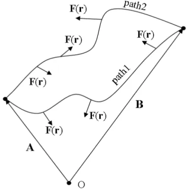
Take a test charge and move it slowly in the F(r) force field from position A to position B on two alternative paths.
Figure 1.1: Integration on two paths
Let us calculate the amount of work done on each path. The force exerted to the test charge by my hand is just opposite of the force field -F(r). If it was not the case, the charge would accelerate. The moving is thought to happen quasi-statically without acceleration.
10
Let us calculate my work for the two alternate paths:
W1 =
B
Z
A
(−F)dr
path1
W2 =
B
Z
A
(−F)dr
path2
(1.11)
In general case W1 and W2 are not equal. However, in some special cases they may be equal for any two paths. Imagine that our force field is such, that W1 and W2 are equal. In this case a closed loop path can be made which starts with path 1 and returns to the starting point on path 2. Since the opposite direction passage turns W2 to its negative, ultimately the closed loop path will result in zero. That special force field where the integral is zero for any closed loop is considered CONSERVATIVE force field.
In formula:
I
F(r)dr= 0 (1.12)
Using the concept of electric field with the formulaF=qEabove equation is transformed:
I
E(r)dr= 0 (1.13)
According to the experience the electric field obeys the law of conservative field. The integral on any closed loop results zero. That also means that curve integral between any two points is independent of the path and solely depends on the starting and final point.
1.7 Voltage and potential
The work done against the force of the electric field is as follows:
WAB =
B
Z
A
(−F)dr=q
B
Z
A
(−E)dr (1.14)
Let us rearrange and divide with q.
UAB = WAB
q UAB =−
B
Z
A
E(r)dr (1.15)
The voltage of pointBrelative toAis given by the formula above. The fact is clear that the voltage is dependent on two points. If the starting point is considered as a reference
point for all the integrals, that specific voltage will be dependent on the final point only.
This one parameter voltage is called the potential.
UB =−
B
Z
ref
E(r)dr (1.16)
Voltages can be expressed as the difference of potentials proven below:
UAB =
−
ref
Z
A
E(r)dr
+
−
B
Z
ref
E(r)dr
=
−
B
Z
ref
E(r)dr
−
−
A
Z
ref
E(r)dr
=UB−UA (1.17) The potential of any point can also be written as follows:
U(r) = −
r
Z
ref
E(r,)dr, (1.18)
The concept of voltage exists always and its value is definite. The value of potential is indefinite because it depends on the reference point too. However this is possible to define a definite potential. The reference point of the integral should be placed to the infinity. This can be done in case of physically real objects when the corresponding improper integral is convergent. The physically real object is by definition such an object which virtually shrinks to a point if one departs infinite far away. The spherical charge arrangement is the only physically real object among those mentioned above. An infinite long cylinder or an infinite plan parallel plate are not physically real, since viewed from infinite it still looks infinite.
1.8 Gradient
The gradient is an operation in vector calculus which generates the electric field vector from the potential scalar field. In general case the formula is as follows:
gradU(r) = ∂U(r)
∂x i+∂U(r)
∂y j+ ∂U(r)
∂z k=−E(r) (1.19) Therefore:
E(r) =−gradU(r) (1.20) In the special case of spherical cylindrical and plane parallel structures the gradient operation is merely a derivation according to the position variable.
E(r) =−dU(r)
dr (1.21)
12
1.9 Spherical structures
1.9.1 Metal sphere
Metal sphere with radius R =0.1m contains Q =10−8As charge. Find the function of the electric field and the potential as the function of distance from the center and sketch the result. Calculate the values of the electric field and the potential on the surface of the metal sphere. Determine the capacitance of the metal sphere.
Metal contains free electrons therefore electric field may not exist inside the bulk of the metal. If there was electric field in the metal the free electrons would move to compensate it to zero very fast. Since there is no electric field inside the metal the total volume of the metal is equipotential. The vector of the electric field is always normal (perpendicular) to the metal (equipotential) surface. The proof of this as follows: If there was an angle different of ninety degrees then this electric field vector could be decomposed to normal and tangential components. The tangential component would readily move the electrons until this component gets compensated. In stationary case all the excess charge resides on the surface of the metal. Therefore a hollow metal is equivalent with a bulky metal in terms of electrostatics. The surface charge density and the surface electric field are proportional to the reciprocal of the curvature radius.
I
S
E(r)·dA= Q
ε0 (1.22)
Gauss’s law is used to solve the problem. We pick a virtual point-like balloon and inflate it from zero to the infinity radius. Inside the metal sphere there is no contained charge in the balloon.
4r2π·E = 0 (1.23)
E = 0 (1.24)
So the electric field inside the metal sphere is zero.
Out of the metal sphere however the contained charge is the amount given in this problem.
4r2π·E = Q
ε0 (1.25)
The electric field can be expressed:
E(r) = Q 4πε0
· 1
r2 (1.26)
On the surface of the metal sphere the electric field comes out if r =R is substituted to the above function
E(R) = Q 4πε0 · 1
R2 = 9·10910−8
0.12 = 9000V
m (1.27)
The potential function can be determined by integrating the electric field:
U(r) =−
r
Z
∞
E(r,)dr,=−
r
Z
∞
Q 4πε0 · 1
r,2dr,= Q 4πε0 ·
r
Z
∞
(− 1
r,2)dr,= (1.28)
= Q
4πε0 1
r, r,=r
r,=∞
= Q
4πε0 1
r − 1
∞
= Q
4πε0 1
r (1.29)
So briefly the potential function out of the metal sphere is as follows:
U(r) = Q 4πε0
1
r (1.30)
On the surface of the metal sphere the potential comes out if r=R is substituted to the above function
U(R) = Q 4πε0
1
R = 9·10910−8
0.1 = 900V (1.31)
Inside the metal sphere the potential is constant due to the zero electric field.
Figure 1.2: Metal sphere
Electric field vs. radial position function Potential vs. radial position function
14
An interesting result can be concluded. Let us divide the formula of the potential and the electric field on the surface.
U(R)
E(R) = Q 4πε0
1
R · 4πε0
Q R2 =R (1.32)
The electric field on the surface is the ratio of the potential and the radius.
E(R) = U(R)
R (1.33)
The result is in perfect agreement with the numerical values.
This result is useful when high electric field is desired. This time ultra sharp needle is used and the needle is hooked up to high potential. By means of this device corona discharge can be generated in air.
Capacitance is a general term in physics which means a kind of storage capability.
More precisely this is the ratio of some kind of extensive parameter over the corresponding intensive parameter. For instance the heat capacitance is the ratio of the heat energy over the temperature. Similarly the electric capacitance is the ratio of the charge over the generated potential. The unit of the capacitance is As/V which is called Farad (F) to commemorate the famous scientist Faraday. Farad as a unit is very large therefore pF or µF is used mostly. Capacitance denoted with C is a feature of all physically real conductive objects. In contrast to this the capacitor is a device used in the electronics with intentionally high capacitance.
U = Q 4πε0
1
R (1.34)
C= Q
U = 4πε0R= 1
9·109 ·1F arad= 110pF (1.35) So the capacitance of the metal sphere is proportional to the radius. It is worth remem- bering that a big sphere of one meter radius has a capacitance of 110pF. The capacitance of the human body is in the range of some tens of pF.
1.9.2 Sphere with uniform space charge density
Uniform space charge density (ρ = 10−6 As/m3) is contained by a sphere with radius R = 0.1 meter. (The charge density is immobile. Imagine this in the way that wax is melted charged up and let it cool down. The charges are effectively trapped in the wax.) Find the function of the electric field and the potential as the function of distance from
the center and sketch the result. Calculate the value of the electric field on the surface of the sphere and the value of the potential on the surface and in the center.
I
S
E(r)·dA= Q
ε0 (1.36)
We pick a virtual point-like balloon and inflate it from zero to the infinity radius. Inside the charged sphere the Gauss’s law is as follows:
4r2π·E = 4r3π 3
ρ
ε0 (1.37)
On the left hand side there is the flux on the right hand side there is the volume of the sphere multiplied with the charge density. Many terms cancel out.
E(r) = ρ
3ε0r (1.38)
The result is not surprising. By increasing the radius in the sphere the charge contained grows cubically the surface area increases with the second power so the ratio will be linear.
Outside the charged sphere the amount of the charge contained does not grow any more only the surface of the sphere continues to grow with the second power.
4r2π·E = 4R3π 3
ρ
ε0 (1.39)
E(r) = ρ 3ε0
R3
r2 (1.40)
The two above equations show that the function of the electric field is continuous, since on the surface of the charged sphere r=R substitution produces the same result.
On the surface of the sphere the numerical value of the electric field can readily be calculated:
E(R) = ρ
3ε0R = 10−6
3·8,86·10−12 ·0.1 = 3762V
m (1.41)
The potential function can be determined by integrating the electric field. First the external region is integrated:
Uout(r) = −
r
Z
∞
E(r,)dr,=−
r
Z
∞
ρ 3ε0
R3
r,2dr,= (1.42)
= ρR3 3ε0
·
r
Z
∞
(− 1
r,2)dr,= ρR3 3ε0
1 r,
r,=r r,=∞
= ρR3 3ε0
1 r − 1
∞
= ρR3 3ε0
1
r (1.43)
16
So briefly the potential function out of the charged sphere is as follows:
Uout(r) = ρR3 3ε0
1
r (1.44)
The surface potential of the sphere is the above function with r=R substitution:
U(R) = ρR2
3ε0 = 10−6·10−2
3·8,86·10−12 = 376V (1.45) Remember that this value should be added to the integral calculated next.
Inside the charged sphere the integral is different:
Uin(r) = U(R) +URr =U(R) +
−
r
Z
R
E(r,)dr,
(1.46)
For simplicity reason only the integral in the parenthesis is transformed first:
URr =−
r
Z
R
ρ
3ε0r,dr,=− ρ 3ε0
r
Z
R
r,dr,=− ρ 3ε0
r,2 2
r.=r r,=R
=− ρ 3ε0
r2 2 − R2
2
(1.47)
Altogether:
Uin(r) = U(R) +URr = ρR2 3ε0 +
− ρ 3ε0
r2 2 − R2
2
= ρ 3ε0
3R2 2 − r2
2
= ρ
6ε0 3R2−r2 (1.48) The final result is:
Uin(r) = ρ
6ε0 3R2−r2
(1.49) The numerical value of the central potential is given by the above equation at r = 0 substitution.
Uin(0) = ρ
6ε0 3R2
= ρR2
2ε0 = 10−6·10−2
2·8,86·10−12 = 564V (1.50)
1.10 Cylindrical structures
1.10.1 Infinite metal cylinder
Infinite metal cylinder (tube) with radius R =0.1m contains ω =10−8As/m2 surface charge density. Find the function of the electric field and the potential as the function
Figure 1.3: Sphere with uniform charge density
Electric field vs. radial position function Potential vs. radial position function of distance from the center and sketch the result. The reference point of the potential should be the center. Calculate the value of the electric field and of the potential on the surface of the metal cylinder.
I
S
E(r)·dA= Q ε0
(1.51) Gauss’s law is used to solve the problem. We pick a virtual line-like tube and inflate it from zero to the infinity radius. Inside the metal cylinder there is no contained charge in the virtual tube.
2rπ·l·E = 0 (1.52)
E = 0 (1.53)
So the electric field inside the metal cylinder is zero.
Out of the metal cylinder however the contained charge is as follows.
2rπ·l·E = 2Rπ·l·ω
ε0 (1.54)
The electric field can be expressed:
E(r) = ωR ε0
· 1
r (1.55)
18
On the surface of the metal cylinder the electric field comes out if r =R is substituted to the above function
E(R) = ωR ε0 · 1
R = ω
ε0 = 10−8
8.86·10−12 = 1129V
m (1.56)
The potential function can be determined by integrating the electric field:
U(r) =−
r
Z
R
E(r,)dr,=−
r
Z
R
ωR ε0 · 1
r,dr,=−ωR ε0
r
Z
R
1
r,dr,=−ωR
ε0 [lnr,]rr,,=r=R=−ωR ε0 ln
r R
(1.57) So briefly the potential function out of the metal cylinder is as follows:
U(r) = −ωR ε0 lnr
R
(1.58) On the surface of the metal cylinder the potential comes out if r =R is substituted to the above function
U(R) =−ωR ε0 ln
R R
= 0V (1.59)
The result is obvious since inside the metal cylinder the potential is constant due to the zero electric field.
Note that the reference point of the potential could not be placed to the infinity because the infinite long cylinder is not physically real object. Therefore the improper integral is not convergent.
1.10.2 Infinite cylinder with uniform space charge density
Uniform space charge density (ρ = 10−6 As/m3) is contained by an infinite cylinder with radius R = 0.1 meter. (The charge density is immobile. Imagine this in the way that wax is melted charged up and let it cool down. The charges are effectively trapped in the wax.) Find the function of the electric field and the potential as the function of distance from the center and sketch the result. Calculate the value of the electric field and the potential on the surface of the cylinder. The reference point of the potential should be the central line.
I
S
E(r)·dA= Q
ε0 (1.60)
Figure 1.4: Metal cylinder
Electric field vs. radial position function Potential vs. radial position function
We pick a virtual line-like tube and inflate the radius from zero to the infinity. Inside the charged sphere the Gauss’s law is as follows:
2rπ·l·E =r2π·l ρ
ε0 (1.61)
On the left hand side there is the flux on the right hand side there is the volume of the cylinder multiplied with the charge density. Many terms cancel out.
E(r) = ρ
2ε0r (1.62)
The result is not surprising. By increasing the radius the charge contained grows with the second power, the surface area increases linearly so the ratio will be linear.
Outside the charged cylinder the amount of the charge contained does not grow any more only the surface continues to grow linearly.
2rπ·l·E =R2π·l ρ
ε0 (1.63)
E(r) = ρ 2ε0
R2
r (1.64)
The two above equations show that the function of the electric field is continuous, since on the surface of the cylinder r=R substitution produces the same result.
20
On the surface of the sphere the numerical value of the electric field can readily be calculated:
E(R) = ρ
2ε0R = 10−6
2·8,86·10−12 ·0.1 = 5643V
m (1.65)
The potential function can be determined by integrating the electric field. First the internal region is integrated: The reference point of the potential will be the center.
Uin(r) = −
r
Z
0
E(r,)dr,=−
r
Z
0
ρ
2ε0r,dr, =− ρ 2ε0
r
Z
0
r,dr,=− ρ 2ε0
r,2 2
r,=r r,=0
=− ρ 2ε0
r2 2
=− ρ 4ε0r2 (1.66)
Uin(r) =− ρ
4ε0r2 (1.67)
The surface potential of the cylinder is the above function with r=R substitution:
Uin(R) =−ρR2
4ε0 =− 10−6·10−2
4·8,86·10−12 =−282V (1.68) Remember that this value should be added to the integral calculated next.
Uout(r) = Uin(R) +URr =Uin(R) +
−
r
Z
R
E(r,)dr,
(1.69)
For simplicity reason only the integral in the parenthesis is transformed first:
URr =−
r
Z
R
ρ 2ε0
R2
r dr,=−ρR2 2ε0
r
Z
R
dr,
r, =−ρR2
2ε0 [lnr,]rr.,=r=R=−ρR2 2ε0 ln
r R
(1.70)
Altogether:
Uout(r) =Uin(R) +URr =−ρR2 4ε0 +
−ρR2 2ε0 ln(r
R)
=−ρR2 4ε0
1 + 2 ln(r R)
(1.71) The final result is:
Uout(r) =−ρR2 4ε0
1 + 2 ln(r R)
(1.72)
Figure 1.5: Cylinder with uniform charge density
Electric field vs. radial position function Potential vs. radial position function
1.11 Infinite parallel plate with uniform surface charge density
Infinite metal plate containsω =10−8As/m2 surface charge density. Find the function of the electric field and the potential as the function of distance from the plate and sketch the result. The reference point of the potential should be the center. Calculate the value of the electric field on the surface of the metal plate.
I
S
E(r)·dA= Q ε0
(1.73) Gauss’s law is used to solve the problem. Pick a virtual drum with base plate area A.
Position the drum with rotational axis normal to the charged plate. The charged plate should cut the drum to two symmetrical parts.
E·2A= ωA
ε0 (1.74)
The absolute value electric field can be expressed:
E = ω
2ε0 = 10−8
2·8.86·10−12 = 564V
m (1.75)
22
The result shows that the electric field is constant in the half space.
The direction of the electric field is opposite in the two half spaces. In contrast to the spherical and cylindrical structures where the radial distance is the position parameter, here a reference direction line will be used.
The potential function can be determined by integrating the electric field in the positive half space:
U(x) =−
x
Z
0
E(x,)dx, =−
x
Z
0
ω 2ε0
dx,=− ω 2ε0
x
Z
0
dx, =− ω 2ε0
[x,]xx,,=x=0 =− ω 2ε0
x (1.76) So briefly the potential function is as follows:
U(x) =− ω
2ε0x (1.77)
Obviously the potential function turns to its negative in the negative half space.
Figure 1.6: Infinite parallel plate with uniform surface charge density
Electric field vs. radial position function Potential vs. radial position function
Note that the reference point of the potential could not be placed to the infinity because the infinite plate is not physically real object.
1.12 Capacitors
Capacitors consist of two plates to store charge. The overall contained charge is zero since the charges on the plates are opposite therefore the electric field is confined to the
inner volume of the capacitor. The capacitance is the ratio of the charge over the voltage generated between the plates. C = QU Three different geometries will be treated below.
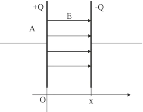
1.12.1/ Parallel plate capacitor
The parallel plate capacitor is made of two parallel metal plates facing each other with the active surface area A. The distance between the plates and the charge are denoted by dand Q, respectively.
Figure 1.7: Parallel plate capacitor
There is homogeneous electric field between the plates, while out of the capacitor there is no electric field. Use the Gauss’s law for a drum-like surface which surrounds one of the plates.
EA= Q
ε0 E = Q
Aε0 (1.78)
To find out the voltage between the plates does not need integration due to the homoge- nous field. U =d·E
U = d·Q
Aε0 (1.79)
And capacitance can be expressed from here.
C =ε0A
d (1.80)
1.12.1 Cylindrical capacitor
The cylindrical capacitor is made of two coaxial metal cylinders. The inner and the outer radii as well as the length are denoted R1, R2 and l, respectively. The coaxial cable is the only practically used cylindrical capacitor.
Let us use the Gauss’s law. A coaxial cylinder should be inflated fromR1 toR2. I
S
E(r)·dA= Q
ε0 (1.81)
24
Figure 1.8: Cylindrical capacitor
E·2rπl = Q
ε0 (1.82)
E = Q 2πε0l · 1
r (1.83)
To find out the voltage the following integral should be evaluated:
U =−
R1
Z
R2
Q 2πε0l · 1
rdr = Q 2πε0l
R2
Z
R1
1
rdr = Q
2πε0l ln(R2
R1) (1.84)
The capacitance can be expressed from here.
C= Q
U = 2πε0l
ln(R2/R1) (1.85)
The above formula shows the obvious fact that the capacitance is proportional to the length of the structure. Because of this the capacitance of one meter coaxial cable is used mostly. This is denoted with cand measured in F/m units. Most coaxial cables represent some 10 pF/m value.
c= Q
U = 2πε0
ln(R2/R1) (1.86)
Figure 1.9: Spherical capacitor
1.12.2 Spherical capacitor
The spherical capacitor is made of two concentric metal spheres. The inner and the outer radii as well as the charge are denoted R1, R2 and Q, respectively.
Let us use the Gauss’s law. A concentric sphere should be inflated from R1 toR2. I
S
E(r)·dA= Q
ε0 (1.87)
E·4r2π= Q
ε0 (1.88)
E = Q 4πε0 · 1
r2 (1.89)
To find out the voltage the following integral should be evaluated:
U =−
R1
Z
R2
Q 4πε0 · 1
r2dr = Q 4πε0
R1
Z
R2
(−1
r2)dr = Q 4πε0
1 r
r=R1
r=R2
= Q
4πε0 1
R1 − 1 R2
(1.90)
26
The capacitance can be expressed from here.
C = Q
U = 4πε0
1 R1 − R1
2
(1.91)
1.13 Principle of superposition
The Gauss’s law can only be used effectively in the three symmetry classes mentioned earlier. If the charge arrangement does not belong to any of those classes the principle of superposition is the only choice. This time the charge arrangement is virtually broken to little pieces and the electric fields of these little pieces are superimposed like point charges.
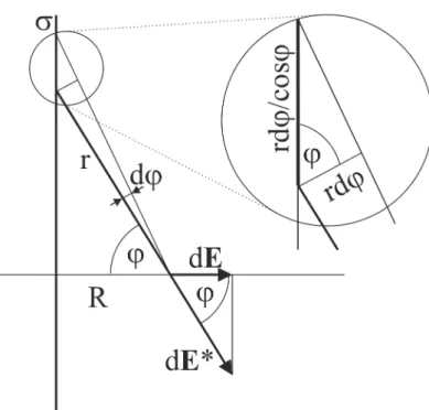
• Find the electric field of a finite long charged filament in the equatorial plane as the function of distance from the filament. The linear charge density is denotedσ.
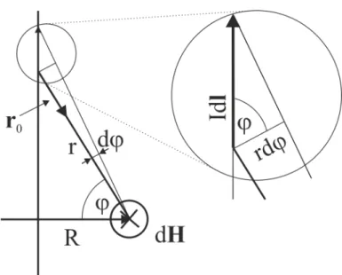
Since the filament is not infinite long Gauss’s law can not be used effectively. The charged filament is divided to little infinitesimal pieces and the electric fields of such pieces are added together. Due to symmetry reasons only the normal components of the electric field are integrated since the parallel components cancel out by pairs. The mathematical deduction of the final formula follows below without close commenting to the transformations. For the definition of the notations refer the figure below:
The infinitesimal contribution of the electric field is calculated as a point charge.
dE∗ = dQ 4πε0 · 1
r2 dQ= rdφ
cosϕσ r= R
cosϕ (1.92)
The infinitesimal charge is contained by the infinitesimal angle.
dE∗ = rdφ cosϕσ 1
4πε0 · 1
r2 = σ 4πε0
1
rcosϕdφ= σ 4πε0
1
Rdφ (1.93)
The electric field of the point charge is projected to the perpendicular direction. The parallel direction components cancel out by symmetric pairs.
dE =dE∗cosφ (1.94)
dE = σ 4πε0
1
R cosφ·dφ (1.95)
The integration is carried out in α half visual angle.
E =
α
Z
−α
dE =
α
Z
−α
σ 4πε0
1
Rcosφ·dφ= σ 4πε0
1 R
α
Z
−α
cosφ·dφ= σ 4πε0
1
R[sinφ]φ=αφ=−α = σ 2Rπε0
sinα (1.96)
Figure 1.10: Principle of superposition
The result of the superposition is the formula below which could not have been attained with Gauss’s law.
E = σ
2Rπε0 sinα (1.97)
If αapproaches ninety degrees the filaments tend to the infinity when using Gauss’s law is an option.
E∞= lim
α→π2 E = σ 2Rπε0
(1.98) Using Gauss’s law the above result can be reached far easier for the infinite long filament.
E∞·2Rπ·l= σl
ε0 (1.99)
E∞= σ
2Rπε0 (1.100)
The results are in perfect match. However the point is that superposition principle can be used in full generality, but it is far more meticulous and tedious than using Gauss’s law if that is possible.
28
Chapter 2
Dielectric materials - Gy¨ orgy H´ ars
Insulators or in other words dielectric materials will be discussed in this chapter. In chapter 1 only metal electrodes and immobile charges are the sources of the electric field. In contrast to metals, insulating materials are lacking of mobile electron plasma therefore the electric field can penetrate the insulators. In terms of phenomenology the insulating material is polarized which means that the material as a whole will become an electric dipole. In terms of microphysical explanation, the overall effects of huge number of elementary dipoles will create the external dipole effect. The elementary dipoles are either generated or oriented by the external electric field.
2.1 The electric dipole
Consider a pair of opposite point charges (+q,− −q). Initiate the vector of separation (s) from the negative to the positive point charge. The following product defines the electric dipole moment:
p=qs [Asm] (2.1)
In order to generate a point-like dipole the definition is completed with a limit transition.
Accordingly the absolute value of the displacement vector shrinks to zero while the charge tends to the infinity such a way that the product is a constant vector. The point- like dipole is a useful model when the distance of the charges is far smaller than the corresponding geometry, for example if a dipole molecule is located in the proximity of centimeter size electrodes.
Force couple is exerted to the dipole by homogeneous electric field. The torque (M) generated turns the dipole parallel to the electric field.
Figure 2.1: Dipole turns parallel to the E filed
M=p×E
Asm· V
m =N m
(2.2) The dipole moment turns into the direction of the electric field spontaneously and stays there. Having reached this position, the least amount of potential energy is stored by the dipole. Obviously the most amount of potential energy stored is just in the opposite position. Let us find out the work needed to turn the dipole from the deepest position to the highest energy.
W =
π
Z
0
M dφ=
π
Z
0
pEsinφ·dφ=pE
π
Z
0
sinφ·dφ=−pE[cosφ]π0 = 2pE (2.3) According to this result the potential energy of the dipole is as follows:
Epot =−p·E (2.4)
This formula provides the deepest energy at parallel spontaneous position and the highest at anti-parallel position. The zero potential energy is at ninety degrees. The difference between the highest and lowest is just the work needed to turn it around.
2.2 Polarization
Take a plate capacitor and fill its volume with a dielectric material. The experiment shows that the capacitance increased relative to the empty case. The explanation behind is the polarization of the dielectric material.
30
Figure 2.2: Plate capacitor with dipole chain
Due to the electric field of the metal plates the atomic dipoles have been arranged like the chains as the figure shows above. Inside the dielectric material the electric effect of dipoles cancel out since in any macroscopic volume equal number of positive and negative charges is present. The exceptions are the two sides of the dielectric material where the uncompensated polarization surface charge densities reside. These uncompensated polarization surface charges are opposite in polarity relative to the adjacent metal plates.
This way the effective total charge is reduced, thus voltage of the capacitor diminished and ultimately the capacitance is increased.
Assume that the insulating material contains n pieces of dipoles per unit volume (1/m3). The surface area and the separation of the plate capacitor is denoted A and d respectively. The total number of dipoles (N) is as follows:
N =Adn (2.5)
The dipoles are located in chains between the metal plates. The number of dipoles in such a chain is the ratio of the distance between the plates (d) and the separation of the dipoles (s). The total number of dipoles (N) can be expressed if the length of the chain is multiplied with the number of chains (c) present in the material:
N = d
sc (2.6)
Let us combine these latter two equations:
Adn= d
sc Ans=c (2.7)
The separation (s) can be expressed as ratio of the dipole moment (p) and the charge of the dipole (q). (In present discussion the absolute values of the quantities are denoted without vector notation.)
s= p
q (2.8)
So the number of chains can be expressed:
c=Anp
q (2.9)
The total polarization surface charge is the product of the number of chains and the uncompensated opposite charge at the end of each dipole chain.
Qp =c(−q) =−Anp (2.10)
Finally the polarization surface charge density (ωp) needs to be expressed:
ωp = Qp
A =−np=−P
As m2
(2.11) Here we introduced the vector of the “polarization (P)”. The sources of this vector are the opposite of the polarization charges. The negative polarity comes from the definition of the electric dipole which points from to minus to the plus in contrast to the direction of the electric field. (Without vector notation the absolute value is meant).
An additional result can also be concluded. The density of dipoles gives rise to the polarization. The formula is valid in three dimensions too.
P =np P=np (2.12)
2.3 Dielectric displacement
Figure 2.3: Plate capacitor with polarized dielectric material
32
The metal plates of the capacitor contain what are called the “free charges”. The free charges are mobile and can be conducted away by means of a wire. In contrast to this the polarization charges are immobile.
In chapter 1 the homogeneous electric field in plate capacitor has been expressed, provided the free surface charge densities (+ωfree, -ωfree) are located on the metal plates.
Ef ree = ωf ree
ε0 ε0Ef ree =ωf ree (2.13)
Here we introduce the vector of the “dielectric displacement (D)”. The sources of this vector are the free mobile charges. (Without vector notation the absolute value is meant).
ε0Ef ree =D=ωf ree
As m2
(2.14) The polarization surface charges (+ωp, -ωp) perform the same way but in opposite di- rection:
Ep = ωp
ε0 ε0Ep =ωp (2.15)
ε0Ep =−P =ωp
As m2
(2.16) The total surface charge density is the sum of the free and the polarization charges:
ωtot =ωf ree+ωp (2.17)
The total charge density is the source of the resulting electric field in the capacitor:
ε0E =D−P (2.18)
D=ε0E+P (2.19)
The last formula has been deduced for one dimensional case. The parameters show up here as they were real numbers. However the result is true in full generality in three dimensions with vectors as well.
D =ε0E+P (2.20)
Note the important fact that the electric field and so the intensity of forces are always reduced in presence of dielectric material.
2.4 Electric permittivity (dielectric constant)
Experiments show that the polarization of some isotropic material is the monotonous function of the external electric field. At external fields of higher intensity the insulating material is gradually saturated. At relatively low levels the function can be considered linear. Our next discussion is confined to the linear range. This case the proportionality is holding between the polarization and the external electric field. In order to make an equation out of the proportionality a coefficient (χ) is introduced.
P=χε0E (2.21)
The coefficient is the permittivity of vacuum (ε0) and the electric susceptibility (χ).
Substitute this equation to the former expression of D vector:
D =ε0E+χε0E=ε0(1 +χ)E=ε0εrE (2.22) Here the relative permittivity (εr) has been introduced:
1 +χ=εr (2.23)
Typical values of the relative permittivity are up to five or so. Very high numbers are technically impossible.
Finally the result to be remembered is as follows:
D=ε0εrE
As m2
(2.24)
2.5 Gauss’s law and the dielectric material
In this section the vector calculus will be used at somewhat higher level.
The divergence operation (div) generates a scalar field which represents the sources of some vector field.
V(r) = Vx(x, y, z)i+Vy(x, y, z)j+Vz(x, y, z)k (2.25)
divV(r) = ∂Vx
∂x + ∂Vy
∂y + ∂Vz
∂z (2.26)
The Gauss Ostrogradsky theorem integrates the divergence to a volume as follows:
I
S
V(r)dA= I
V
(divV)dV (2.27)
34
Let us generate the divergence of the equation discussed earlier in this chapter:
D =ε0E+P (2.28)
divD =div(ε0E) +divP (2.29) The sources or in other words the divergences are the corresponding volume charge den- sities (ρfree, ρtot, ρp) in general. Earlier in this chapter the surface charge densities have been discussed in details for the case of the plate capacitor. Accordingly the following relations are plausible:
divD=ρf ree div(ε0E) = ρtot divP=−ρp (2.30)
Gauss Ostrogradsky theorem generates integral form from the relations above:
I
S
DdA=Qf ree I
S
(ε0E)dA=Qtot I
S
PdA=−Qp (2.31)
The left hand side integral is the well-known form of Gauss’s law with D vector. This expresses that the flux of D vector on a closed surface (S) equals the amount of the contained free charges. The integral in the middle expresses that the flux of ε0E vector equals the total amount of any contained charges. Finally the right hand side states that the flux of the polarization Pvector equals the opposite of the polarization charges contained by the S surface.
2.6 Inhomogeneous dielectric materials
Consider two different dielectric materials with plane surface. The plane surfaces are connected thus creating an interface between the insulators. This structure is subjected to the experimentation.
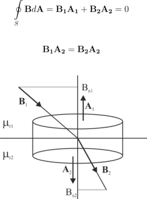
First the D field is studied.
The interface is contained by a symmetrical disc-like drum with the base areaA. The upper and lower surface vectors are A1 and A2 respectively.
A1 =−A2 |A1|=|A2|=A (2.32)
The volume does not contain free charges therefore the flux of the D vector is zero.
I
S
DdA=D1A1+D2A2 = 0 (2.33)
D1A2 =D2A2 (2.34)
Figure 2.4: D field at the interface of different dielectric materials
The operation of dot product contains the projection of theDvectors to the direction of A2 vector which is the normal direction to the surface. The subscript n means the absolute value of the normal direction component.
D1nA2 =D2nA2 (2.35)
Once we are among real numbers the surface area cancels out readily.
D1n =D2n (2.36)
According to this result the normal component of D vector is continuous on the inter- face of dielectric materials.
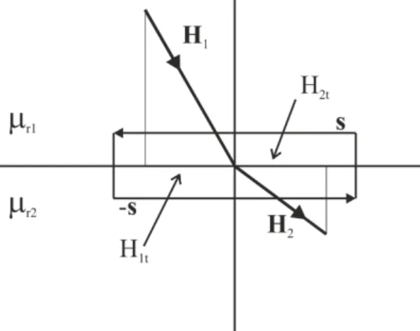
Secondly the electric field E is the subject of analysis.
Figure 2.5: E field at the interface of different dielectric materials 36
The interface is surrounded by a very narrow rectangle-like loop with sections parallel and normal to the surface. The parallel sections of the loop are s and –s vectors. The normal direction sections are ignored due to the infinitesimal size. The closed loop integral of the E in static electric field is zero.
I
g
Edr =sE1+ (−s)E2 = 0 (2.37)
sE1 =sE2 (2.38)
The operation of dot product contains the projection of the E vectors to the direction of s vector which is the tangential direction to the surface. The subscript t means the absolute value of the tangential direction component.
sE1t=sE2t (2.39)
Once we are among real numbers the length of the tangential section cancels out readily.
E1t=E2t (2.40)
According to this result the tangential component of the E vector is continuous on the interface of dielectric materials.
2.7 Demonstration examples
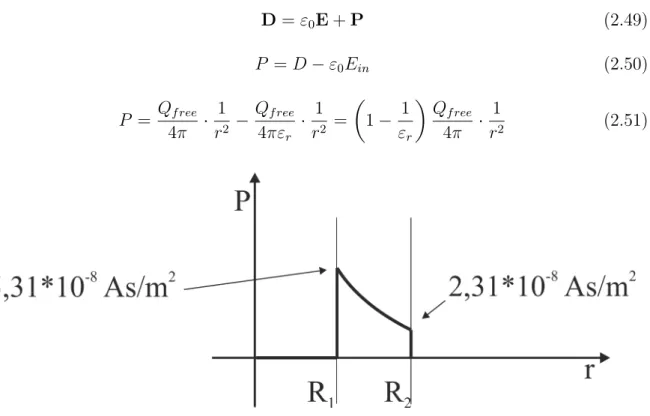
2.7.1
A metal sphere with radius (R1 = 10cm) contains free charges (Qf ree = 10−8As).
The metal sphere is surrounded by an insulating layer (εr = 3) up to the radius (R2 = 15cm). Find and sketch the radial dependence of D, E and P vectors. Determine the numerical peak values in the break points and find the amount of the polarization charge.
The first parameter to deal with is the D vector because the normal component is continuous on the interface of dielectric materials. Let us use the Gauss’s law.
I
S
DdA=Qf ree (2.41)
Figure 2.6: Metal sphere surrounded by insulating layer
Inside the metal sphere all the parameters are zero only out of the metal sphere is of interest.
4r2π·D=Qf ree (2.42)
D= Qf ree
4π · 1
r2 (2.43)
Figure 2.7: The absolute value of D vs. radial position function 38