CLASSIFICATION OF TIGHT CONTACT STRUCTURES ON SMALL SEIFERT FIBERED L-SPACES

(1)

arXiv:1601.05059v2 [math.GT] 7 Jul 2017

IRENA MATKOVI ˇC

Abstract. The Ozsv´ath-Szab´o contact invariant is a complete classification invariant for tight contact structures on small Seifert fibered 3-manifolds which areL-spaces.

1. Introduction

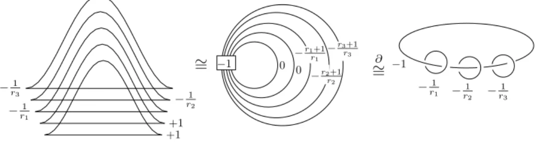
By small Seifert fibered 3-manifold we refer to Seifert fibration over the sphere S²with three singular fibers, standardly given asM(e0;r1, r2, r3) wheree0∈Zand ri∈Q∩(0,1) withr1 ≥r2≥r3. For a surgery presentation of this manifold, see the right diagram of Figure 1.

L-spaces (by definition, Heegaard Floer homology lens spaces) among Seifert fibered manifolds are geometrically characterized by absence of transverse contact structures [12, Theorem 1.1], which is essential for our classification. The restriction can be simply described in terms of the Seifert constants: L-spaces are all manifolds with e0 ≥ 0 and with e0 ≤ −3, while for e0 = −1,−2 some explicit numerical inequalities (see Subsection 4.4) are imposed on the triple (r1, r2, r3).

Problem to classify tight contact structures up to contact isotopy is usually asked for prime atoroidal manifolds; the first because tight contact structures respect connected sum decomposition of 3-manifolds, the second because an embedded essential torus is a known source of infinitely many non-isotopic tight structures.

Small Seifert fibered manifolds, beside hyperbolic ones, share these properties. On the other hand, the existence question for Seifert manifolds has been completely an- swered by Lisca-Stipsicz [13]: only the ones which belong to a one-parameter family of (2n−1)-surgeries on the torus knotT2,2n+1 (equivalently, which are orientation preserving diffeomorphic to M(−1;¹₂,_2n+1ⁿ ,_2n+3¹ ) for some n ∈ N) do not admit any tight structure. Classification then arises from the comparison of bounds: the lower bound is obtained constructively by contact surgery complemented with the use of invariants, and for the upper bound the convex surface theory is applied.

The main invariant in the classification of tight Seifert fibered manifolds is the maximal twisting number (that is, the difference between the contact framing and the fibration framing, maximized in the smooth isotopy class of a regular fiber) – applied in convex surface theory, it allows one to give upper bounds on the number of tight structures. By the results of Wu [20] all tight contact structures when e0≤ −2 have negative maximal twisting, while fore0≥0 they are all zero-twisting;

in the work of Ghiggini [3] the negative maximal twisting is further related to the existence of transverse contact structures. This, in the case ofL-spaces, results in

2010Mathematics Subject Classification. 57R17.

Key words and phrases. Seifert fibered 3-manifolds, tight contact structures, contact Ozsv´ath- Szab´o invariant, convex surface theory.

1

(2)

a simple division: maximal twisting is equal to zero when e0≥ −1, and has value

−1 when e0 ≤ −2. The fixed maximal twisting of a regular fiber in all the cases gives some unique contact structure on the complement of singular fibers relative to boundary, pushing the classification into tubular neighborhoods of the three singular fibers.

The classification whenever e0 6= −1 is then finished by Legendrian surgery construction – the diagrams are simply given by Legendrianization of standard presentation of Seifert manifold; this is done in [20, 4, 3] for e06=−2,−1,0, e0≥ 0, e0=−2, respectively. In particular, all these tight structures are Stein fillable, and classified by the first Chern class of their fillings [10], equivalently by their Spin^c structure, or closer to the present context by their contact Ozsv´ath-Szab´o invariants [17].

The remaining case ofM(−1;r1, r2, r3) has been partly addressed already in [5].

Here, the constructive side needs to be attacked differently because of the existence of non-fillable tight structures. Invoking that all tight structures are zero-twisting [3], Lisca-Stipsicz gave a uniform description of all possible tight structures by certain surgery diagrams.

Proposition 1.1. [12, Proposition 6.1]Each tight contact structure with maximal twisting equal to zero on the small Seifert fibered spaceM(−1;r1, r2, r3)is given by

one of the surgery presentations of Figure 1 left.

This reduces the classification problem to the recognition of tightness and isotopies between the finite collection of structures, listed by the associated Thurston- Bennequin and rotation numbers.

−_r¹₃

−_r¹₂

−_r¹₁

+1 +1

∼=

−^r³_r⁺¹

3

−^r²_r⁺¹₂

−^r¹_r⁺¹₁ 0 0

−1 ∂

∼= ⁻¹

−_r¹₁ −_r¹₂ −_r¹₃

Figure 1. Contact structures onM(−1;r1, r2, r3), followed by the smoothened surgery diagram of the underlying 3-manifold and its standard presentation; when referring to them as 4-manifolds, we assume inverse slam-dunks to be done.

The underlying topological question, classification of oriented 2-plane fieldsξ∈Ξ up to homotopy is given by their induced Spin^c structure t_ξ together with the 3- dimensional invariant d3(ξ). (Recall that π0(Ξ) can be identified with homotopy classes of maps [M, S²], which can be through Pontryagin-Thom construction given by framed links in M; here link up to oriented cobordism represents the class in H1(M;Z), equivalentlyt_ξ, while the framing corresponds to the Hopf invariant as a 3-dimensional obstruction for homotopies between plane fields.)

To detect tightness, we basically use the Ozsv´ath-Szab´o contact invariant [16], implicitly expecting all tight structures to have non-vanishing one. But we address it indirectly, by showing the sufficient condition of Lisca-Stipsicz.

2

(3)

Theorem 1.2. [12, Theorem 1.2]If for a contact structureξof Figure 1 on Seifert fiberedL-spaceM =M(−1;r1, r2, r3) the equality d3(ξ) =d(M,t_ξ) holds, then its contact invariantc(M, ξ)∈HFd(−M,t_ξ)does not vanish.

Then, to confirm overtwistedness of all non-detected structures and to obtain the isotopies between tight ones, as always, convex surface theory is applied.

The observations accumulate in the confirmation of [18, Conjecture 4.7].

Theorem 1.3. LetMbe a small Seifert fiberedL-space of the formM(−1;r1, r2, r3).

Then a contact structure ξ on M is tight if and only if it is given by a contact surgery presentation of Figure 1 and its 3-dimensional invariant d3(ξ) is equal to thed-invariantd(M,t_ξ). Moreover, two tight structuresξ1 andξ2onM are contact isotopic if and only if their inducedSpin^c structurest_ξ₁,t_ξ₂ are isomorphic.

Expressed in terms of the Ozsv´ath-Szab´o contact invariant all tight structures on small Seifert fiberedL-spaces satisfy the following.

Corollary 1.4. Let ξbe a contact structure on small Seifert fiberedL-spaceM = M(e0;r1, r2, r3). Thenξis tight if and only if its contact invariantc(ξ)∈HFd(−M,t_ξ) is nonzero. Moreover, two tight structuresξ1andξ2 are isotopic if and only if their contact invariantsc(ξ1), c(ξ2)coincide, if and only if their inducedSpin^c structures t_ξ₁,t_ξ₂ are isomorphic.

Proof. If there are less than three singular fibers, the manifold considered is a lens space. Here as well as whene06=−1, all tight structures are Stein fillable according to previous results [2, 7, 20, 4, 3]. By that and Theorem 1.3 above, tight structure on any consideredM has non-vanishing contact invariant.

The fillable structures are classified by the contact invariant due to Plamenevskaya [17]. In fact, for L-spaces the non-trivial contact invariant of ξ is the unique generator ofHFd(−M,t_ξ), henceξis the only tight representative of its induced Spin^c structure. Its 3-dimensional invariantd3(ξ) is specified as the absolute grading of

the contact invariant, which equalsd(M,t_ξ).

Our result reduces the classification problem to a well-understood computation of invariants. Although our method does not result in the number of tight structures on a given small Seifert manifold, the problem is translated to a completely combinatorial (so not geometric) count. Indeed, in any special case the number can be easily determined by, say, a computer calculation (as here both d3 and d are computable, and the Spin^c structure can be given as an element ofH1). What is more, since there is a surgery presentation of considered contact manifolds, we have a very explicit description of tight structures.

Remark 1.5. In contrast to the cases with e0 6= −1, not all tight structures on M(−1;r1, r2, r3) are fillable. Whenever r1+r2 < 1, in the language of [9]

for manifolds of special type, the existence of Stein filling is even topologically obstructed. And as all contact structures of the form given by Figure 1 are known to be supported by open books with planar pages [12], the theorem of Wendl [19]

implies they are not fillable at all. Most manifolds withr1+r2 ≥ 1 admit Stein fillable as well as non-fillable tight structures, as specified in [14].

Overview. In Section 2 we explain the structure of our proof, and review main concepts behind it. Then in Section 3 we illustrate the suggested approach by

3

(4)

reproving the classification on Mp := M(−1;¹₂,¹₂,¹_p) [5]. Technical details are given in the last two sections. In Section 4 we establish paths of characteristic covectors separating the presentations into classes with the same contact invariant.

Finally in Section 5, with the help of convex surface theory, the presentations of the same class are realized to be contact isotopic, more, the failure of the tightness criterion is related to overtwistedness.

Acknowledgement. I am indebted to Andr´as Stipsicz for his insightful mentoring.

2. Outline of the proof

Following the classification scheme given in the Introduction, we need a construction, a method to detect tightness (Subsection 2.1), and finally a proof that it is complete (that is, a way to recognize overtwistedness and isotopies between possibly different presentations of the same contact structure; Subsection 2.2).

By Proposition 1.1, to construct tight structures onM(−1;r1, r2, r3) which is an L-space, the contact surgery presentations of Figure 1 suffice. This gives a finite collection of contact structures, on which we need to run the following two-step analysis.

2.1. Detect tightness. In order to detect tightness we examine the equality between the 3-dimensional homotopy invariant d3 of the contact structure and the d-invariant of the induced Spin^c structure (according to Theorem 1.2). The advan- tage of this condition over the Ozsv´ath-Szab´o contact invariant is that these two invariants are easily computable. They can be described in terms of characteristic covectors on plumbings bounded by±M, which brings them into the same picture (as presented below).

We exploit two 4-manifolds, naturally arising as fillings of ourM, one given by the smoothened surgery diagram (Figure 1 middle) – call itX – and another given by standard smooth presentation of Seifert fibration (Figure 1 right) – sayW =WΓ

as we can think of it as a simple plumbing along the graph Γ. They are related byX#CP²∼=W#2CP². Further, the plumbing description of−M will play the central role in what follows. Call it WΓ^′ where Γ^′ stands for the plumbing graph, dual to Γ.

Now, the 3-dimensional invariant of the contact bundleξcan be directly read off from the surgery presentationd3(ξ) = ¹₄(c²(X, J)−3σ(X)−2b2(X))+#(+1-surgeries) [1, Corollary 3.6], wherec(X, J) stands for the characteristic element, determined by the ξ-induced almost complex structure J of X\{a point in each +1-handle}.

While the d-invariant corresponds to the reversely oriented−M (which bounds a negative-definite plumbing) together with an induced Spin^c structure t_ξ. It is realized by the characteristic 2-cohomology class, which gives Spin^c cobordism from S³ to (−M,t_ξ) whose associated map in Heegaard Floer homology decreases absolute grading the least. These are recognized by full paths [15, Subsection 3.1]. To establish some terminology let us recollect.

Full path. Assume that Γ^′ is a negative definite plumbing with at most one bad vertex. At-tuple (K1, . . . , Kt) of characteristic covectors onWΓ^′ forms a full path if its elements are connected by the following 2 PD steps: for some vertexv with hKi, vi=−v·v, the vector Ki+1is given by Ki+1=Ki+ 2 PD(v). (In particular, all its elements induce the same Spin^c structure on the boundary∂WΓ^′ =−M as they differ only by twice generators ofH²(WΓ^′,−M;Z). Further, their (common)

4

(5)

degree can be computed by the formula ¹₄(K_i²+|Γ^′|).) The path ends either by some characteristic vectorK which exceeds the boundsv·v ≤ hKi, vi ≤ −v·v at somev∈Γ^′– we will say that it drops out. Otherwise the path reaches the proper ends in the initial vectorK1satisfyingv·v+ 2≤ hK1, vi ≤ −v·v for allv∈Γ^′and the terminal vectorKtsatisfyingv·v≤ hKt, vi ≤ −v·v−2 for allv∈Γ^′ – such ending full path according to [15] determines a non-trivial element ofHFd(−M).

Embedding into blown-upCP².

p l₂

l₃ l1

l

−→

0

−1 +1 0

0

⊆CP²#CP² → · · · → Γ ⁻¹

−1

−1 Γ^′

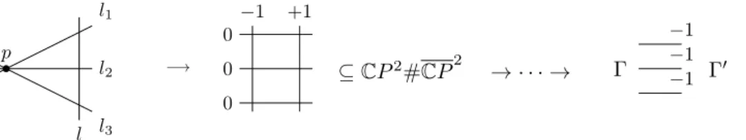
Figure 2. Construction of the 4-manifold R = CP²#nCP²; at the end, the two plumbings are glued together along the exceptional spheres from the last blow-up of each singular fiber, and (not shown) all regular fibers.

According to [13, Lemma 4.2] we can embed M as a hypersurface in a closed oriented 4-manifold R so that R\ν(M) = WΓ∪WΓ^′. The configuration of both intersection graphs Γ,Γ^′ is obtained by blowing-up the initial linesl1, l2, l3⊂CP²: l1∩l2∩l3={p}, andl⊂CP²:p /∈l (see Figure 2).

Denote standard generators of H2(R;Z) as follows: h(h² = 1) for the initial CP¹⊂CP², and ei (e²_i =−1) for exceptional curves. Then the above description of the embeddingWΓ∪WΓ^′ ֒→R gives:

• {z= center of Γ} 7→e1

• {z^′= center of Γ^′} 7→h−e2−e3−e4

• {xi= first vertex of the legLi⊂Γ} 7→h−e1−ei+1−P

ej fori= 1,2,3

• {v vertex,v6=z, z^′, xi} 7→ej−P

ek, for example {x^′_i= first vertex of the dual legL^′_i⊂Γ^′} 7→ei+1−P

ek fori= 1,2,3.

We will refer to Γ as the manifold side and Γ^′ as the dual side. Throughout, we will follow the convention that primed notation belongs to the dual graph: apart from the special vertices denoted above, let vⁱ_j be thej^th vertex ofLi andv_jⁱ^′ the j^th vertex ofL^′_i.

Tightness criterion. We haved3 given by a characteristic covector onWΓ,dgiven by a characteristic covector on WΓ^′, and what is more, we can glue these two plumbings along a rational homology sphere M, giving blown-up CP² (calledR).

Having a characteristic covector c on R, which agrees with the ones providing d3

anddonWΓ andWΓ^′ respectively, the equalityd3(ξ) =d(M;t_ξ) can be rewritten asc²=σ(R). This can be understood as geometrization of Theorem 1.2.

Theorem 2.1. [13, Theorem 3.3]LetM =M(−1;r1, r2, r3)be anL-space. Then a sufficient condition for a contact structureξonM to be tight (even forc(M, ξ)6= 0) is in the existence of a characteristic cohomology class c∈H²(R;Z)such that:

5

(6)

(i) d3(ξ) = ¹₄((c|WΓ)²−3σ(WΓ)−2b2(WΓ)) + 1(c|WΓ corresponds toc(X, J));

(ii) c|WΓ′ belongs to an ending full path onWΓ^′(gives rise to a class ofHFd(−M,t_ξ));

(iii) c²=σ(R).

(1)

−1

(rot²₀−1)

−a²₀= tb²₀ (rot¹₀−1)

−a¹₀= tb¹₀

(rot³₀−1)

−a³0= tb³0

−a¹₁= tb¹₁−1 (rot¹₁)

−a²₁= tb²₁−1 (rot²₁)

−a³1= tb³1−1 (rot³₁)

−a¹_k₁= tb¹_k₁−1 (rot¹_k₁)

−a²_k₂= tb²_k₂−1 (rot²_k₂)

−a³_k₃= tb³_k₃−1 (rot³_k₃)

...

−a³_k^′′

3 −a³₁^′

−a¹_k^′′

1 −a¹₁^′

−a²_k^′′

2 −a²₁^′

−a³₀^′

−a²₀^′

−a¹₀^′

−2

...

z=e1

x1=h−e1−e2−P ei . . . x2=h−e1−e3−P

ei . . . x3=h−e1−e4−P

ei . . .

z^′=h−e2−e3−e4

x^′₁=e2−P ei . . . x^′₂=e3−P

ei . . . x^′₃=e4−P

ei . . . Figure 3. Plumbing graph Γ (left) and its dual Γ^′ (right) with denoted self-intersections and evaluations of characteristic covector c, (·) =hc, vi, on the manifold side; the central and the first vertices on legs are given in generating classes ofH2(R;Z).

For a given surgery presentation, the conditions read as follows (see Figure 3):

(i) conWΓis determined byc(X, J), on generators ofH2(X) evaluated as rotation numbers (central blow-up decreases all the (neighboring) values by 1);

(ii) is to be checked given the constraints from (i);

(iii) we can give c as PD(c) = αh+P

αiei where α, αi ∈ {±1}, by construction fulfilling the equalityc²=σ(R).

Technically speaking, given a tuple (cv)v∈Γ ofc-evaluations (cv) =hc, vias in (i), we list all possible±1 distributions in the expression PD(c) of (iii), and calculate corresponding values on Γ^′. We know that these different Γ^′-evaluations are for each given surgery presentation only different representatives of the same full path – they all describe the same Spin^c structure on the boundary. We continue this path towards its ends so that we connect to it all the characteristic covectors which can be obtained by allowed 2 PD steps. Taking all (cv)-tuples, this results in the separation of the characteristic lattice into components; denote themPξ according to the contact structureξthey belong.

In this language, Theorem 1.3 takes the following working form.

Theorem 2.2. The contact structureξ on M(−1;r1, r2, r3)given by surgery diagram is tight if and only if its full path Pξ properly ends in the initial and terminal vector. Two such contact structures ξ1, ξ2 are isotopic if and only if their paths Pξ1,Pξ2 meet (hence, coincide).

2.2. Prove overtwistedness and describe contact isotopies. Finally, to close our classification we need that the zero elements (drop-outs) correspond to overtwistedness, and for the second part of Theorem 1.3 (Theorem 2.2) that elements

6

(7)

giving the same HFd(M)-generator (sharing the same path) are actually contact isotopic.

Here, convex surface theory comes in. We need to translate contact surgeries back into convex decomposition. Natural convex decomposition of the manifoldM separates the three singular tori from the rest of the manifold. Then the coefficients in the continued fraction expansions of the three surgeries, along with the chosen stabilizations determine basic slice decompositions of the three tori.

Contact surgery. Contact surgery in addition to ordinary surgery prescribes for the contact structure to be preserved in the complement of a tubular neighborhood of the core link, while the extension to glued-up tori needs to be tight. The extended contact structure is determined by the boundary slope [7, Theorem 2.3], given by the surgery coefficient. Contact surgery diagrams [1] encode a basic slice decomposition of the glued-up solid torus. The slope uniquely determines continued fraction blocks.

Concretely, writing out the continued fraction expansion of the surgery coefficient

−1 ri

=−aⁱ₀− 1 . ..−_−a¹i

ki

= [aⁱ₀, . . . , aⁱ_k_i]

(we use the convention of [5] withaⁱ_j≥2), continued fraction blocks are toric annuli in the layering of the solid torus with boundary slope [aⁱ_k_i, . . . , aⁱ₀], cut out by pairs of tori of slopes [aⁱ_k_i, . . . , aⁱ_j+1−1] and [aⁱ_k_i, . . . , aⁱ_j−1] (the outermost being [aⁱ_k_i, . . . , aⁱ₀], and the innermost −1). In a surgery diagram, they are represented in a chain of pushed-off knots with appropriate integral surgery coefficients (after turning into±1 surgeries, captured by Thurston-Bennequin invariants). The remaining ambiguity in the signs of the basic slices within each continued fraction block is reflected in the choice of stabilizations of the corresponding Legendrian knot (equivalently their differences as their total number is determined by the surgery coefficient), so given by its rotation number. In the translation positive and negative basic slices in the decomposition of a continued fraction block correspond to positive and negative stabilizations (down- and up-cusps) of corresponding Legendrian knot. The loss of basic slice ordering in the transition is explained by the shuffling property [7, Lemma 4.14] of basic slices within a single block.

What we need is to relate steps in the full path with appropriate state traversals, and drop-outs to non-tight basic slice configurations.

In other words, we have set up two ways to describe rotation numbers. Provided the surgery coefficient is fixed, they can be equally given by either the number of negative basic slices (up-cusps) or the number of negative signs on the generators forming the corresponding part of the dual leg. Then the nice thing – to be shown – is that the full path connections reflect the known behavior of basic slices.

3. First example

We illustrate our strategy on small Seifert fiberedL-spacesMp:=M(−1;¹₂,¹₂,¹_p).

The classification on these manifolds was first obtained by Ghiggini-Lisca-Stipsicz in [5]; wherever applicable, we use their notation. First we describe tight structures onMp using Theorem 1.3, then we prove Theorem 1.3 in this special case.

Claim 3.1. ManifoldMpadmits exactly three tight contact structures up to isotopy.

7

(8)

The finite collection of contact structures, given by Figure 1, can be encoded in the following table of invariants:

surgery coefficient tb rot(|rot| ≤ −tb−1)

+1 −1 0

−1 −2 rot1∈ {−1,1}

−1 −2 rot2∈ {−1,1}

−1 −p rot3∈ {−p+ 1,−p+ 3, ..., p−1}.

As an application of the Theorem, the tightness and isotopies can be recognized solely from the induced Spin^c structures and the two invariants. In our case these are as follows.

d3(ξ) = ¹₄(c²(X, J)−3σ(X)−2b2(X)) +q

=¹₄((0,0,rot1,rot2,rot3)Q⁻¹_X (0,0,rot1,rot2,rot3)^T −3·(−1)−2·5) + 2.

So, for mixed (rot1,rot2) = (±1,∓1), the d3 is always zero, as for (rot1,rot2) = (±1,±1) it runs through the values{^2−p₄ , ...,^−2+3p₄ }by the step±1 as rot3increases.

There are exactly four Spin^c structures for eachp(as|H1(Mp;Z)|= 4):

H1(−Mp;Z) =

*

µ, µa, µb, µc;







1 1 1 1

1 p 0 0

1 0 2 0

1 0 0 2











 µ µa

µb

µc





= 0 +

=

hµb; 4µb= 0i ∼=Z4 forpodd

hµb, µc; 2µb= 2µc= 0i ∼=Z2⊕Z2 forpeven.

They can be given by the set{t1 =t₄+µb,t₂ =t₄+µc,t₃ =t₄+µa,t₄}. And corresponding four characteristic 2-cohomology classes, realizingd(−Mp,t_i), are on the generators ofH2(WΓ^′) given by:

(0) (2)

(0)

(0) (0)

...

K1

(0) (0)

(2)

(0) (0)

...

K2

(0) (0)

(0)

(0) (0) (2)

...

K3

(0) (0)

(0)

(0) (0)

...

K4

Therefore:

d(−Mp,t_i) = max

c1(s)²+|Γ^′|

4 ;s∈Spin^c(WΓ^′),s|−Mp=t_i

=





0 i= 1,2

p−2 4 i= 3

p+2 4 i= 4 Applying Theorem 1.3, the above computations already give that for distinct rot1,rot2all structures are tight, and belong to two different isotopy classes, while for equal rot1,rot2the only tight triples are (±1,±1,∓(p−1)) and they are isotopic to each other. This proves Claim 3.1.

Claim 3.2. Theorem 1.3 holds forMp.

We show this following the two-step analysis described in Section 2.

3.1. Detect tightness. The condition we use to recognize tight structures among all (Mp, ξ) presented by surgery diagrams of Figure 1 is an existence of the characteristic covectorc as in Theorem 2.1.

8

(9)

We givec as PD(c) = αh+P

αiei where α, αi ∈ {±1}, and such that (ci) = hc, xii= roti−1. Concretely, thec-evaluations on Γ belong to one of the following.

(1)

−1

(−2) or (0)

−2 (−2) or (0)

−2

(−p) or (−p+ 2) or ... or (p−2)

−p

z=e1

x1=h−e1−e2−e5

x2=h−e1−e3−e6

x3=h−e1−e4−Pp+5 7 ei

Then, for each such (α, αi) we computec|Γ^′, and check how its full path ends.

−2 −2 −2

−2

...

z^′=h−e2−e3−e4

x^′₁=e2−e5

x^′₂=e3−e6

x^′₃=e4−e7, e7−e8, . . . , ep+4−ep+5

Below we table all possible (α, αi) for each given triple (c1, c2, c3). We will make explicit how some c|Γ^′ drop out, and connect the others to the right initial and terminal vector. Also, we will emphasize the appearance of the same characteristic covectorsc|Γ^′ in some pairs ofc-triples.

First observe that (on the level of paths) the order of signs on generators of each leg is unimportant, as they can be shuffled using ±2 PD(v^′)-steps forhc, v^′i=±2.

Then there are essentially only two different sign-vectors (α, αi) for a chosen c- triple, differing in the sign of h. The two are connected by ±2 PD(z^′), applied whenhc, z^′i=±2. Notice that all these different sign configurations belong to the same surgery presentation.

In the light of the previous paragraph, we record only the number of positive and negative signs on exceptional generators of each leg. Write {m+, n−}i when there arem positive and nnegative generators ofLi (counted without hande1);

not to be confused with vectors of signs which record exact sign configuration on corresponding generators. In addition, let (h+)(c1,c2,c3) and (h−)(c1,c2,c3) denote any of sign configurations which belongs to (c1, c2, c3) and has positive, negative respectively, sign onh. Look separately at the cases with the same, and later with the distinct (c1, c2).

c3 (−2,−2, c3) (0,0, c3)

(h−) (h+) (h−) (h+)

{1+,1−}1 {0+,2−}1 {2+,0−}1 {1+,1−}1

{1+,1−}2 {0+,2−}2 {2+,0−}2 {1+,1−}2

p−2 {p+,0−}3 {(p−1)+,1−}3 {p+,0−}3 {(p−1)+,1−}3

p−4 {(p−1)+,1−}3 {(p−2)+,2−}3 {(p−1)+,1−}3 {(p−2)+,2−}3

... ... ... ... ...

−p {1+,(p−1)−}3 {0+, p−}3 {1+,(p−1)−}3 {0+, p−}3

For (−2,−2, c3), c3 ∈ {p−4, ...,−p}, there exists a configuration (h, e2, e3, e4) = (−,−,−,−) which drops out: hc, z^′i=h−h−e2−e3−e4, h−e2−e3−e4i=−4.

Similarly, (0,0, c3), c3∈ {p−2, ...,−p+2},drops out at (h, e2, e3, e4) = (+,+,+,+).

Therefore, the paths possibly end only for the triples (−2,−2, p−2) and (0,0,−p).

Furthermore, we observe that (−2,−2, p−2) and (0,0,−p) belong to the same full path because configurations (h−)(−2,−2,p−2)and (h+)_(0,0,−p)give the same characteristic vector (0’s on the third leg, and (h, e4) : (−,+)↔(+,−) with the same

9

(10)

evaluation onz^′=h−e2−e3−e4). This proves also that their (common) path indeed ends, namely atK3(given by (h, e4, e7, ..., ep+4, ep+5) = (−,−,−, ...,−,+) for (0,0,−p)) on the initial side and at−K3(as (h, e4, e7, ..., ep+4, ep+5) = (+,+,+, ...,+,−)

for (−2,−2, p−2)) on the terminal.

c3 (−2,0, c3) (0,−2, c3)

(h−) (h+) (h−) (h+)

{1+,1−}1 {0+,2−}1 {2+,0−}1 {1+,1−}1

{2+,0−}2 {1+,1−}2 {1+,1−}2 {0+,2−}2

p−2 {p+,0−}3 {(p−1)+,1−}3 {p+,0−}3 {(p−1)+,1−}3

p−4 {(p−1)+,1−}3 {(p−2)+,2−}3 {(p−1)+,1−}3 {(p−2)+,2−}3

... ... ... ... ...

−p {1+,(p−1)−}3 {0+, p−}3 {1+,(p−1)−}3 {0+, p−}3

Sign configurations adapted to anyc-triple with distinctc1andc2build a connected part of (one of the two) full paths. Indeed, let us see how these parts patch together into a path. Fork∈ {1, ..., p−1}, we have

(h+)(−2,0,p−2k) =

c|Γ′

(h−)(0,−2,p−2k−2) ≡

c|Γ

(h+)(0,−2,p−2k−2) =

c|Γ′

(h−)(−2,0,p−2k−4)

where the first and the last equality denote the same characteristic covector on Γ^′, while the middle equivalence means (different sign distributions of) the same presentation. This separates all characteristic vectors arising from presentations with mixed (c1, c2) into two full paths. One starting atK1(as −h−e2+e5+e3+ e6+e4+e7+· · ·+ep+5for (−2,0, p−2)) and ending at−K2(as +h−e2−e5+e3−e6− e4−e7−· · ·−ep+5for (−2,0,−p)) or−K1(as +h+e2−e5−e3−e6−e4−e7−· · ·−ep+5

for (0,−2,−p)). The other starting atK2(as−h+e2+e5−e3+e6+e4+e7+· · ·+ep+5

for (0,−2, p−2)) and ending at−K1(as +h+e2−e5−e3−e6−e4−e7− · · · −ep+5

for (0,−2,−p)) or−K2(as +h−e2−e5+e3−e6−e4−e7−· · ·−ep+5for (−2,0,−p)).

The two terminal possibilities depend on parity ofp(odd or even).

In conclusion, translated back into rotation numbers we have obtained the following paths of tight structures, each sharing the same invariants:

• (−1,−1, p−1) and (1,1,−p+ 1) (Spin^c=t₄+µa, d3=^2−p₄ )

• (−1,1, p−1) and (1,−1, p−3) and (−1,1, p−5) and ... (Spin^c =t₄+µb d3= 0)

• (1,−1, p−1) and (−1,1, p−3) and (1,−1, p−5) and ... (Spin^c=t₄+µc, d3= 0) 3.2. Prove overtwistedness and describe contact isotopies. In our (simplest possible) cases with boundary slopes ¹_k, k∈Z, there is a single continued fraction block for each special fiber. Contact surgery presents direct translation between positive and negative stabilizations (down- and up-cusps) of core Legendrian un- knots and positive and negative basic slices in the decomposition of a continued fraction block with slopes−1 and −k. The generators forming the corresponding leg (and by that, the dual vertices) in the plumbings above can be thought of as another way of layering solid torus intokslices.

We need contact topological interpretation for the steps in full paths.

First, the unimportance of sign permutations in the legs coincide with the shuffling of basic slices within a single continued fraction block [7, Lemma 4.14]. More- over, [5, Section 6] provides sufficient isotopy moves between contact structures presented by different surgery diagrams. Let us spell this out. Since the moves in [5] are given by the matrices of signs whose coefficients are qⁱ_j, the number of

10

(11)

positive basic slices in the j^th continued fraction block of the i^th leg, in our case only (q¹₀, q₀², q₀³), we rewrite previously obtained paths of tight structures in this language, changing rotation numbers toqⁱ₀’s:

• (0,0, p−1) and (1,1,0)

• (0,1, p−1) and (1,0, p−2) and (0,1, p−3) and ...

• (1,0, p−1) and (0,1, p−2) and (1,0, p−3) and ...

Now, we notice that conditions which caused a full path to drop out, and so prevented our tightness criterion to work, exactly agree with condition for which overtwistedness can be proved. And finally, there are contact isotopies between pairs of surgery presentations which share the same path. Let us recite.

Proposition 3.3. [5, Propositions 6.3, 6.1 & 6.4] Let a contact structure on Mp

be given by(q₀¹, q²₀, q₀³)as above. Then the triples(1,1, q³₀)withq³₀6= 0and(0,0, q³₀) with q₀³6=p−1 present overtwisted structures. Between other presentations, there are following contact isotopies:

(1,0, q³₀)≃

(0,1, q₀³+ 1)whenq³₀< p−1

(0,1, q₀³−1)whenq³₀>0 and (1,1,0)≃(0,0, p−1).

Problems in general. Examples shown above are special in several ways. In general, it can happen that the full path associated to some presentation (cv)v∈Γdrops out, although all characteristic covectors computed from (α, αi)-configurations which restrict to (cv)v∈Γ satisfy the boundsv·v≤ hc, vi ≤ −v·v for allv∈Γ^′. Also, not all the steps in a full path need to be presentable, that is, arising from some tuple of rotation numbers. (For examples of such paths, look at the two “applications”

in [13].) That said, we need to find out how the (subsequent) presentations of the same path are related, when neither of their characteristic covectors on Γ^′coincides (Corollary 4.14). Finally, we need new conditions for overtwistedness (Proposition 5.1) and isotopies (Proposition 5.2), which will explain such behavior of full paths.

4. Characteristic covectors, tightness, and full paths

In Subsection 2.1, we have associated characteristic covectors on Γ^′to any given surgery presentation. Here we investigate their full paths. Namely, how these paths end, and which presentations share the same path. In order to do so, we first observe that certain 2 PD-steps do not change the presentation (Subsection 4.1).

Then, we explore the only remaining central step – concretely, we explain it on the level of homology generators (Subsection 4.2). In the following Subsections, we are then concerned with the associated change in c|Γ, whether this new c|Γ comes from some presentation and when it leads to the end of the path (Subsection 4.3).

Moreover, we describe (in Subsection 4.4) the first presentable c|Γ (or the end of path) following any possible starting point.

Notation 4.1. We describe a characteristic 2-cohomology class c ∈ H²(R;Z) as PD(c) = αh+Pαiei where α, αi ∈ {±1}. In the following, vectors of signs correspond to parts of the coefficient-vector (α, αi), covering generators of (usually) a single Γ- or Γ^′-vertex.

To a single vertex we often refer by its self-intersection. When a vertex is written out in generating classes, these are called starting, middle and last, according to the position; explicitly, ifv=es−Pl

j=s+1ej, thenesis starting,elis last, and all

11

(12)

others are middle. On legs, the starting generator of a vertex and the last generator of the previous vertex coincide.

Presentability will be assigned to dual vectors and it means that the corresponding manifold side arises from a contact presentation, that is, the manifold-side evaluations can be expressed by rotation numbers as in Figure 3.

Let our starting point be a characteristic vector which comes from a contact presentation, and which satisfiesv·v≤ hc, vi ≤ −v·v (otherwise we have already dropped out). We will follow the path only in one direction – towards the initial vector. Recall that the corresponding step is given by−2 PD(v) for somev with hc, vi=v·v, and the vector we aim at satisfiesv·v+ 2≤ hc, vi ≤ −v·v. Everything could be verbatim repeated with opposite signs in the direction of the terminal vector.

4.1. Steps on legs. First, we observe that steps taken forv6=z^′never change the presentation considered, neither the path drops out at any of these vertices. (To the remaining casev=z^′ we dedicate Subsection 4.2.)

Lemma 4.2. Characteristic vectorscandc−2 PD(v), v6=z^′,hc, vi=v·v,always belong to the same surgery presentation.

Proof. As these vertices (v ∈ Γ^′, v 6= z^′) are described by v = ei−P ej, the evaluation of characteristic covectorcreaches the self-intersection when presenting generators all admit the same sign as in the vertex. So, −2 PD(v) changes their signs from (+−· · · −) to (−+· · ·+). But this change has no effect on the evaluation ofc on any of the Γ-vertices.

Indeed, from the way how the exceptional classes are chosen we see that each ej starts some new vertex, either one on the manifold side or one on the dual side. So, the starting and the last generator ofv are non-starting on the manifold side, while all its middle generators are starting (and last) generators of manifold vertices. Hence, the restriction ofcto the generators of v evaluates trivially on Γ, hc|v,Γi= 0, and is therefore independent of sign.

Since these (manifold-side) evaluations directly correspond to rotation numbers, by neither of these moves we switch between presentations.

Lemma 4.3. All drop-outs occur in the center z^′ =h−e2−e3−e4 of the dual star.

Proof. We notice that all the vertices in legs of Γ^′ are formed by exactly as many generators (ej’s) as the value of their self-intersections. Hence, there is no way to drop out at any of them. So, the only possible drop-out happens at z^′ when the signs of generatorshand e2, e3, e4 are all the same ((+ + ++) or (− − −−), and

hc, z^′i=±4).

In sum, we may assume the initial conditionv·v+ 2≤ hc, vi ≤ −v·v is violated only at the central vertex z^′ – such vector can be easily reached by finishing all possible−2 PD-steps on legs, which either sweep out the problem or transfer it to the center. (As each −2 PD-step pushes the problem to the neighboring vertices, we are successively completing the steps, as long as we do not run into a vertexv which despite of the−2-change does not evaluate asv·v, or we reach the end of the leg.) In particular, neither non-central vertex is of the form (+− · · · −).

12

(13)

4.2. Central step. After the above reduction, covector c either drops out at z^′, presents the initial vector or, it reaches self-intersection at z^′. For the latter, the generators formingz^′=h−e2−e3−e4take values: either (+−−−) or (−+−−), up to reordering the legs. The−2 PD-step taken next changes exactly these generators by twice (−+ ++). In the first case we stay in the same presentation, as the step only switches the signs in the pairs (h, ei), i = 2,3,4, preserving the evaluation on all the influenced manifold vertices, x1, x2, x3. In the second case, we can (on the level of generators) instead of simply adding −2z^′ to the given description of PD(c), first change the sign configuration, without changing the dualc|Γ^′ and with controlled (seen later) change on the manifold sidec|Γ, and then do the−2 PD-step as above, not influencing the manifold side.

Algorithm 4.4 (Central step or turn). Whenever we arrive, after possibly renum- bering the legs, atc with (h, e2, e3, e4) = (−+−−) andhc, vi 6=v·v for allv6=z^′, the next step in the full path is given by the characteristic covector c as follows.

Denoting vertices ofL^′₁ by{v₀^′, . . . , v_k^′′

1} and their generators asv_i^′=eⁱ₁−Pli

j=2eⁱ_j witheⁱ_l_i =eⁱ⁺¹₁ and e⁰₁ =e2, define PD(c) = PD(c) + 2h−2e2 and modify it as follows:

fori∈ {0, . . . , k^′₁} ifhc, eⁱ₁i 6=hc, eⁱ₁i: forj∈ {2, . . . , li} ifhc, eⁱ_ji= +1 :

PD(c) = PD(c)−2eⁱ_j & stop ifhc, eⁱ₁i=hc, eⁱ₁i: stop.

Then add−2z^′to so obtained sign configuration PD(c).

To prove well-definedness, we need that such reformulation always exists (the inner loop in our Algorithm always stops, Lemma 4.5) and that uniqueness, ensured by always taking the first positive generator (chosen ordering of the inner loop), can be explained by the independence of order, at least as far as contact presentations are concerned (Lemma 4.6).

Lemma 4.5. Every characteristic vector cΓ^′ with PD(c|z^′) = (−+−−) can be achieved by another distribution of signs, with positive sign onh; it is associated to a different manifold vector (possibly non-presentable).

Proof. Starting at the centerz^′, the two distributions are given by (−+−−) and (+− −−). The switch of theh-sign with the opposite sign of e2, does not impose any change into the second and the third dual leg. For the first leg, the appropriate adaptation of signs, which results in the same dual evaluation, exists because of exclusion of any (+− · · · −)-configurations (that is, the assumption hc, vi 6= v·

v for anyv6=z^′).

Lemma 4.6. As a sign on one middle generator of a dual vertex is changed, all of them need to be changed (independent of order) before we get back into presentable.

A turn of the last generator can result in a presentable vector only when all prior middle generators are negative.

Proof. For a covector to be presentable, all dual vertices have to have same-signed middle generators, because these generators on the manifold side are forming a chain of−2’s, zero being their only possible rotation number.

For the second claim, suppose on the contrary the middle signs on some v^′ are positive. Changing the sign of its last generator (from positive to negative) forces

13

(14)

a switch of all the signs in the following chain (if any) of dual −2’s (to preserve dual evaluations). Then, this influences the evaluation on the next non-(−2) dual vertex w^′, which can be corrected by changing one of its later generators from positive to negative. If the middle generators of w^′ are already negative or if we get them all negative by the current turn, we have found (independent of further changes) a manifold-side vertex which starts at positive (second last) generator in v^′ and has all further signs negative. If by the change of one middle generator not all of them are negative, the vector is non-presentable by the first part. If all generators ofw^′ are positive, and we turn the last one, we need to repeat the same argument with w^′ in place ofv^′. It remains to check whether we could get presentable result by correcting only starting and last generators of all following (necessarily, fully positive) dual vertices. But if not before, the process ends in non-presentable, giving (+− · · · −) on the last manifold vertex.

To sum up, the central turns are the only significant steps in following possible changes on manifold vectors, and by that, in presentations. We may assume that after each central turn also all−2 PD-steps on legs are finished.

4.3. On turning sequences and presentability. To begin, notice how to recognize the ends of a full path.

Lemma 4.7. If after a central step, covectorc on the starting dual vertices evaluates as their self-intersection,hc, x^′_ii=x^′_i·x^′_i:

• on at most one leg, we have arrived at the initial end;

• on two legs, the full path continues;

• on all three legs, this causes a drop-out.

Proof. The maximal starting dual evaluations tell us on how many legs we need further −2 PD-steps. The evaluation on z^′,hc, z^′i, right after a central turn is +2.

If further turns are needed for one leg only we do not reach−2 central evaluation again and the corresponding vector is initial; with two we get back tohc, z^′i=−2 and we continue with another central turn; three gives a drop-out in (h, e2, e3, e4) =

(− − −−).

Corollary 4.8. A presentationξ, whosePξ properly ends, necessarily admits a leg, starting in a fully positive vertex. (If presentation corresponds to the initial vector, there are two fully positive starting vertices.)

Proof. For PD(c) take a sign configuration which evaluates on manifold vertices according to the rotation numbers ofξ, which takes minus sign onh, and for which hc, v^′i 6=v^′·v^′ for allv^′∈Γ^′\{x^′_i;i= 1,2,3}. (This is the stage right after a central turn.) As in Lemma 4.7 above, there is a leg, say L1, for which hc, x^′₁i 6=x^′₁·x^′₁. We prove that on this leghc, x1i=a¹₀−2 holds, that is, the generators ofx1 (apart fromh, e1) are positive.

Write outx1 ash−e1−e2−e5− · · · −eJ. The signs on the generators up to eJ−1 are positive as otherwise we would have shuffled the negative sign to e5 by

−2 PD-steps on consecutive dual vertices of square −2 (resulting in hc, x^′₁i =−2 forx^′₁=e2−e5). The positivity ofeJ follows from presentability via the following claim.

Claim. A presentable covector on neither dual vertex takes the form (+− · · · −+).

14

(15)

Proof. A proof of this fact is basically the same as the second part of the proof of Lemma 4.6. Suppose on the contrary, there is such a dual vertex; it is not the last vertex of the dual leg, because it would give the last vertex on the manifold side with self-intersection−2 and +2c-evaluation. But then, every non-(−2) dual vertex further on the dual leg needs to have again negative middle signs (otherwise we have found a manifold vertex, starting in the negative sign of the previous non-(−2) with all following generators positive) and positive last one (because of (+− · · · −) exclusion). After all, ending in the impossible last dual vertex.

Since also (+− · · · −)-configuration on any dual vertex, exceptx^′_i,is excluded by hc, v^′i 6=v^′·v^′, and since middle generators of any dual vertex are same-signed, we get thateJ is positive. It is a middle generator of a dual vertex starting in positive

eJ−1.

The leg with fully positive starting vertex is the one which in the reordering of Algorithm 4.4 takes role ofL1. When we wish to emphasize according to which leg in the actual structure the central step is done, we refer to it as a turn ofLi.

Since the evaluation of characteristic covector on Li-vertices changes only by turns ofLi, we may separately study their influence.

Lemma 4.9. Letcbe a presentable non-initial characteristic covector. Assume that it evaluates on the vertices of some legL= (−a0,−a1, . . . ,−aj,−aj+1, . . . ,−ak)as follows:

hc, Li= (a0−2, a1−2, . . . , aj−2, aj+1−2−2nj+1, . . . , ak−2−2nk) wherek≥j, nj+1, . . . , nk≥0 andnj+1 >0.

The path runs into the next possibly presentable covector¯c only after 1 + 1 + (a1−1) + (a2−1)(a1−1) +· · ·+ (aj−1−1)· · ·(a1−1)turns of L, in:

h¯c, Li= (−a0,−a1+ 2, . . . ,−aj+ 2, aj+1−2nj+1, . . . , ak−2−2nk).

Proof. To be illustrative, we explicitly write out all the generators involved in the first few turns. Below are the two sides, L1 and L^′₁, in homology generators; the

∗-symbol stands for truncation only.

L1: x1=h−e1−e2−e5− · · · −eJ−1− eJ

eJ− eJ+1

eJ+1− eJ+2

. ..

eK−1−eK−eK+1− ∗ L^′1: x^′1=e2− e5

. ..

eJ−2− eJ−1

eJ−1−eJ−eJ+1− · · · − eK

∗

In this notation, the starting part ofL1and the evaluation ofcon it take values:

L1= (−J+ 3,−2, . . . ,−2

| {z }

K−J−1

,−T,−S,∗) andhc, L1i= (J−5,0, . . . ,0, M, N,∗).

15

(16)

By the first turn, according to the Algorithm, we change generators up to eJ

– it does not influence further dual vertices, but a new vector can be presentable only when all the middle generators eJ, ..., eK−1 are same-signed. Therefore, in order to (possibly) reach presentable vector again we have to repeat turning of this particular leg (K−J)-times. Resulting manifold vector is of the form (−J+ 3,0. . . ,0, M + 2, N,∗), its presentability depends on the (+2)-changed manifold vertexeK−1−eK−eK+1− ∗.

In terms of generators, we have reached another presentation exactly wheneK- sign is negative. The positive eK-sign, on the other hand, requires another turn, but this forces some further changes to preserve the dual. Namely, we need to change signs on generators of the following chain of −2’s, and one (without loss of generality, first) middle generator afterwards. The resulting vector is not necessarily presentable, provided the starting point was, it depends on presentability of the vertex starting in the (last changed) middle generator (+2 rotation change). But if it is, the new presentation is (−J+ 3,0, . . . ,0,−T+ 2, N+ 2,∗); for this, we need to turn this leg (K−J+ 1)-times.

Continuing in the same manner, we trace similar behavior at all levels. Con- cretely. We are successively turning fully positive vertices, which influences the evaluation on the following manifold vertex by +2. If the result is presentable, we have finished. Otherwise, the following vertex was also fully positive, at the moment its evaluation is minus self-intersection, and it will have turned under the influence of another turn of the previous vertex. For that we need to bring the previous vertex back to maximal rotation, using (again) influence of the previous vertices on leg. But notice that each vertex is influenced only by turns of the vertex just before it. Therefore, to come from maximal rotation through minus self-intersection to minimal rotation on some vertexvk+1, we need to influence it by two turns of its first previous vertex vk. This in turn is obtained by (ak−1) turns of its previous vertex vk−1, by first to get from minus self-intersection to minimal rotation, and then by the step of +2 to maximal rotation. This explains the number of steps and

finishes the proof.

Obviously, the leg (its vertices with self-intersections) together with the sign configuration (in presentable, rotation numbers) determine when the leg is turned.

In particular, it specifies the gaps between the subsequent turnings of the same leg, when some other leg needs to be turned in order for the path to continue. Actually, the reverse also holds.

Lemma 4.10. A form of a leg together with a distribution of signs on its generators is completely described by the sequence of its turns.

Proof. As before, separately state (and argue for) the first step.

Claim. Between two subsequent turnings of the same legLthere are always either a0−2 ora0−1 turnings of other two legs.

Proof. Remember that all generators (but possibly last) of the starting manifold vertex on the turning leg are positive. Since by each turn of other legs we change starting evaluation by +2 (through the change ofh-sign from negative to positive), the gap is determined by the number of generators of the starting vertex. Its variation by one is due to whether the dual vertex following −2’s is also fully

negative after theL-turn.

16