minimum difference representations
Zolt´an F¨uredi1∗ and Ida Kantor2†
1 Alfr´ed R´enyi Institute of Mathematics, Budapest, Hungary (e-mail: z-furedi@illinois.edu)
2 Charles University, Prague (e-mail: idasve@gmail.com)
Abstract
Every graphG= (V, E) is an induced subgraph of some Kneser graph of rankk, i.e., there is an assignment of (distinct)k-setsv7→Avto the verticesv∈V such thatAu and Av are disjoint if and only ifuv∈E. The smallest suchkis called theKneser rankofG and denoted byfKneser(G). As an application of a result of Frieze and Reed concerning the clique cover number of random graphs we show that for constant 0 < p <1 there exist constantsci=ci(p)>0,i= 1,2 such that with high probability
c1n/(logn)< fKneser(G)< c2n/(logn).
We apply this for other graph representations defined by Boros, Gurvich and Meshulam.
A k-min-difference representationof a graph Gis an assignment of a set Ai to each vertexi∈V(G) such that
ij ∈E(G) ⇔ min{|Ai\Aj|,|Aj\Ai|} ≥k.
The smallestk such that there exists a k-min-difference representation of G is denoted byfmin(G). Balogh and Prince proved in 2009 that for everykthere is a graph Gwith fmin(G) ≥ k. We prove that there are constants c001, c002 > 0 such that c001n/(logn) <
fmin(G)< c002n/(logn) holds for almost all bipartite graphsGonn+nvertices.
0Keywords and Phrases: random graphs, Kneser graphs, clique covers, intersection graphs.
2010 Mathematics Subject Classification: 05C62, 05C80. [Furedi_Kantor_final.tex]
Submitted to??? Printed on November 12, 2018
∗Research was supported in part by grant (no. K116769) from the National Research, Development and Innovation Office NKFIH, by the Simons Foundation Collaboration Grant #317487, and by the European Research Council Advanced Investigators Grant 267195.
†Supported by project 16-01602Y of the Czech Science Foundation (GACR).
1
arXiv:1701.08292v1 [math.CO] 28 Jan 2017
1 Kneser representations
A representation of a graph G is an assignment of mathematical objects of a given kind (intervals, disks in the plane, finite sets, vectors, etc.) to the vertices of G in such a way that two vertices are adjacent if and only if the corresponding sets satisfy a certain condition (intervals intersect, vectors have different entries in each coordinate, etc.). Representations of various kinds have been studied extensively, see, e.g., [7], [10], the monograph [15], or from information theory point of view [13]. The representations considered in this paper are assignments v 7→ Av to the vertices v ∈ V of a graph G = (V, E) such that the Av’s are (finite) sets satisfying certain relations.
The Kneser graph Kn(s, k) (for positive integers s ≥ 2k) is a graph whose vertices are all thek-subsets of the set [s] :={1,2, . . . , s}, and whose edges connect two sets if they are disjoint. An assignment (A1, . . . , An) for a graph G = (V, E) (where V = [n]) is called a Kneser representation of rank k if each Ai has size k, the sets are distinct, and Au and Av
are disjoint if and only ifuv∈E.
Every graph onnvertices with minimum degreeδ < n−2 has a Kneser representation of rank (n−1−δ). To see that, define theco-star representation (A01, . . . , A0n) ofG. For every i∈ V(G), let A0i be the set of the edges adjacent to i in the complement of G (this is the graphGwithV(G) =V(G) andE(G) = V(G)2
\E(G)). We haveA0i∩A0j = 1 ifij 6∈E(G), otherwise A0i∩A0j = 0, and the maximum size of A0i is n−1−δ(G). To turn the co-star representation into a Kneser representation add pairwise disjoint sets of labels to the sets A01, . . . , A0nto increase their cardinality to exactlyn−1−δ(G). The resulting setsA1, . . . , An are all distinct, they have the same intersection properties asA01, . . . , A0n, and form a Kneser representation ofG of rankn−1−δ(G).
Let G(n) denote the set of 2(n2) (labelled) graphs on [n] and let G(n, k,Kneser) denote the family of graphs on [n] having a Kneser representation of rank k. G ∈ G(n, k,Kneser) is equivalent to the fact thatG is an induced subgraph of some Kneser graph Kn(s, k). We have
G(n,1,Kneser)⊆ G(n,2,Kneser)⊆ · · · ⊆ G(n, n−1,Kneser) =G(n).
LetfKneser(G) denote the smallestk such thatGhas a Kneser representation of rankk. We have seen that fKneser(G) ≤ n−δ. We show that there are better bounds for almost all graphs.
Theorem 1. There exist constants c2> c1>0 such that for G∈ G(n) with high probability c1
n
logn < fKneser(G)< c2
n logn. We will prove a stronger version as Corollary 12.
2 Minimum difference representations
In difference representations, generally speaking, vertices are adjacent if the represent- ing sets are sufficiently different. As an example consider Kneser graphs, where the vertices are adjacent if and only if the representing sets are disjoint. There are other type of repre- sentations where one joins sets close to each other, e.g., t-intersection representations were investigated by M. Chung and West [6] for dense graphs and Eaton and R¨odl [7] for sparse graphs. But these are usually lead to different type of problems, one cannot simply consider the complement of the graph.
This paper is mostly focused on k-min-difference representations (and its relatives), de- fined by Boros, Gurvich and Meshulam in [5] as follows.
Definition 2. Let G be a graph on the vertices [n] = {1, . . . , n}. A k-min-difference repre- sentation (A1, . . . , An) of G is an assignment of a setAi to each vertexi∈V(G) so that
ij ∈E(G) ⇔ min{|Ai\Aj|,|Aj\Ai|} ≥k.
Let G(n, k,min)be the set of graphs with V(G) = [n]that have a k-min-difference represen- tation. The smallest ksuch that G∈ G(n, k,min) is denoted by fmin(G).
The co-star representation (which was investigated by Erd˝os, Goodman, and P´osa [8] in their classical work on clique decompositions) shows that fmin(G) exists and it is at most n−1−δ(G).
Boros, Collado, Gurvits, and Kelmans [4] showed that many n-vertex graphs, including all trees, cycles, and line graphs, the complements of the above, and P4-free graphs, belong to G(n,2,min). They did not find any graph with fmin(G) ≥ 3. Boros, Gurvitch and Meshulam [5] asked whether the value of fmin over all graphs is bounded by a constant.
This question was answered in the negative by Balogh and Prince [3], who proved that for everykthere is an n0 such that whenevern > n0, then for a graph Gon nvertices we have fmin(G)≥kwith high probability. Their proof used a highly non-trivial Ramsey-type result due to Balogh and Bollob´as [2], so their bound onn0 is a tower function ofk.
Our main result is a significant improvement of the Balogh-Prince result. Let G(n, n) denote the family of 2n2 bipartite graphs Gwith partite setsV1 and V2,|V1|=|V2|=n.
Theorem 3. There is a constant c >0 such that for almost all bipartite graphsG∈ G(n, n) one has fmin(G)≥cn/(logn).
Let H be a graph on logn vertices with fmin(H) ≥ clogn/(log logn). One of the basic facts about random graphs is that almost all graphs onn vertices contain H as an induced subgraph. The following theorem is an easy consequence of this fact together with Theorem 3.
Corollary 4. There is a constant c >0 such that almost all graphsG onn vertices satisfy fmin(G)≥ clogn
log logn.
3 On the number of graphs with k–min-dif representations
3.1 The structure of min-dif representations of bipartite graphs
Analogously to previous notation, G(n, k,min) (and G(n, n, k,min)) denotes the family of (bipartite) graphs G with n labelled vertices V (partite sets V1 and V2, |V1| =|V2| =n, respectively) withfmin(G)≤k. Our aim in this Section is to show that there exists a constant c >0 such that |G(n, n, k,min)|=o(2n2) if k < cn/(logn). This implies that for almost all bipartite graphs on n+n verticesfmin(G)≥cn/(logn).
A k-min-difference representation (Ai :i∈ V) of G is reducedif deleting any element x from all sets that contain it yields a representation of a graph different fromG. Note that
|Ai\Aj| −1≤ |(Ai\x)\(Aj\x)| ≤ |Ai\Aj|
so the graphG0corresponding to thek-representation (Ai\x:i∈V) has no more edges than G,E(G0)⊆E(G). There is a natural partition of the elements ofS
Ai: for every∅ 6=I ⊆[n], we have the subset (T
i∈IAi)∩(T
j6∈IAj) whereAj is the complement of the setAj. We call these subsetsatoms. If ak-min-difference representation is reduced, then no atom has more thankelements. It follows that the ground setS
Aiof a reduced representation of ann-vertex graph has no more thank2n elements. Lemma 5 improves on this observation.
Lemma 5. Let G be a graph with n vertices and (A1, . . . , An) a reduced k-min-difference representation of G. Then [
Ai≤2e(G)k≤kn2.
Proof. Define the sets Ai,j := Ai \Aj in the cases ij ∈ E(G), and |Ai \Aj| = k. Let S:=S
Ai,j. The number of elements inS is bounded above by the quantity |E(G)| ·2k. We claim thatS=S
Ai. Otherwise, if there is an elementx∈(S
Ai)\S, then the representation can be reduced, (Ai\x:i∈V) defines the same graph as (Ai :i∈V). 2
The upper bound in Lemma 5 can be significantly improved for bipartite graphs.
Lemma 6. Let G ∈ G(n, n) be a bipartite graph with n + n labeled vertices, G ∈ G(n, n, k,min). Let (A1, . . . , An) and (B1, . . . , Bn) be the sets representing the two parts.
If (A1, . . . , An, B1, . . . , Bn) is a reduced k-min-difference representation of G, then
[ Ai
∪[
Bi≤4kn.
Proof. Suppose that|A1| ≤ · · · ≤ |An|and |B1| ≤ · · · ≤ |Bn|. LetA:=S
Ai and B:=S Bi, S:=A∪B. Define
A0 :=
n−1[
i=1
(Ai\Ai+1). (1)
A A
A A
i+1A
1 2
n i
... ...
... ...
A’
Figure 1: |A1| ≤ · · · ≤ |An|in a min-dif representation when{1,2, . . . , n} is independent
For each i, the inequality |Ai\Ai+1| ≤ |Ai+1\Ai|follows from the assumption that |Ai| ≤
|Ai+1|. The vertices in each part of G form an independent set, so for each i, we have
|Ai\Ai+1| ≤k−1. Hence |A0| ≤(n−1)k.
If x ∈ Aα \Aβ for some α < β, then there is an index i such that x ∈ Ai\Ai+1 and therefore x∈A0. In other words, ifx ∈Aα\A0 and α < β then x∈Aβ. Therefore the sets Ai\A0 form a chain (see Figure 1),
A1\A0 ⊆A2\A0 ⊆ · · · ⊆An\A0.
Treat the other part of G analogously: define B0 and note the same bound on its size, and note that the setsBi\B0 form a chain.
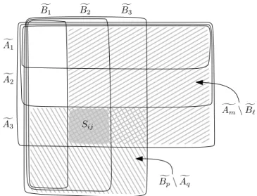
Let us define D=S\(A0∪B0). We will prove that there are at most 2(n+ 1) sets of the formAm\B` and Bp\Aq, each of cardinality k, covering D. ThereforeD contains at most 2(n+ 1)k elements. For each 1 ≤i ≤n, let us define Afi =Ai∩D and fBi = Bi∩D. Let Af0 =Bf0 =∅ and A]n+1 =B]n+1 =D. The sets Af0,Af1, . . . ,Afn,A]n+1 form a chain, same for Bf0,Bf1. . . ,Bfn,B]n+1. The elements ofDbelong to (n+1)2atoms (as defined in the beginning of this section), many of them possibly empty, corresponding to the squares in Figure 2.
For eachi, j, 1≤i, j≤n+1, (i, j)6= (n+1, n+1), the atomSi,j is defined as (fAi\A]i−1)∩ (Bfj \B]j−1). Since the representation is reduced, no elements from the atomSi,j can be left out, so e.g.,S1,1 =∅. It follows that either there are some m and `such that |Am\B`|=k and the atomSi,j belongs in Am\B` (here n≥m≥i≥1 andj > `≥1), or there are some p, q such that |Bp\Aq|=k and the atomSi,j is in Bp\Aq. Since|gAm\Bf`| ⊆Am\B`, we have|gAm\Bf`| ≤k in the first case. Likewise in the second case,|Bfp\Afq| ≤k. In Figure 2, the first option corresponds to a rectangle containing theSi,j cell and the upper-right corner, with all the squares in this rectangle together containing only at mostkelements. The second
Bf1 Bf2 Bf3
Af1
f A2
Af3 Sij
gAm\Bf`
f Bp\Afq
Figure 2: The elements ofS\(A0∪B0) split into (n+ 1)2 atoms.
option corresponds to a similar rectangle with only at most kelements in it, containing the Si,j square and the lower-left corner.
Call a subrectangle gAm \Bf` critical if |Am \B`| = k, and similarly Bfp \Afq is critical if|Bp \Aq| =k. Our argument above can be reformulated that every (nonempty) cell Si,j
is covered by a critical rectangle. This implies that in each row one can find at most two critical rectangles that cover all non-empty atoms in it. This yields the desired upper bound
|D| ≤2(n+ 1)k.
Finally, altogether|S| ≤ |A0|+|B0|+|D| ≤4kn. 2
3.2 Counting reduced matrices
Let S be a set of size |S| = 4kn. In this subsection we give an upper bound for the number of sequences (A1, . . . , An) of subsets of S satisfying the following two properties
(P1) |A1| ≤ · · · ≤ |An|,
(P2) |Ai\Ai+1| ≤k−1 (for all 1≤i≤n−1).
Let M be the 0-1 matrix that has the characteristic vectors of the sets A1, . . . , An as its rows (in this order). The positions in M where an entry 1 is directly above an entry 0 will be calledone-zero configurations, while the positions where a 0 is directly above a 1 will be called zero-one configurations. A column in a 0-1 matrix is uniquely determined by the locations of the one-zero configurations and the zero-one configurations unless it is a full 0 or full 1 column. We count the number of possible matrices M by filling up the n×(4kn) entries in three steps.
Each one-zero configuration corresponds to an i < nand to an element x∈Ai\Ai+1. A setAi+1\Ai can be selected in at most
4nk 0
+· · ·+ 4nk
k−1
<(4en)k
ways (n > k≥1). Do this for eachi < n, altogether we have less than (4en)knways to write in the one-zero configurations intoM.
Select in each column the top 1. If there is no such element in a column we indicate that it is blank, a full zero column. There are at most n+ 1 outcomes for each column, altogether there are at most (n+ 1)4kn possibilities. Fill up with 0’s each column above its top 1. Define A0 ⊂S as in (1),A0 :=Sn−1
i=1(Ai\Ai+1). We have|A0| ≤kn. The columns of Mthat correspond to the elements ofS\A0 have a (possibly empty) string of zeros followed by a string of ones. We almost filled up Mand we can finish this process by selecting the remaining zero-one configurations.
There may be several zero-one configurations in a single column. Each of them has a unique (closest, or smallest indexed) 1 above them. That element 1 is already written in into our still partially filledM, because that element 1 (even if it is the top 1 element) belongs to a unique one-zero configuration. This correspondence is an injection. So there are at most P
i|Ai\Ai+1| ≤ kn zero-one configurations in the columns corresponding to A0 which are not yet identified. There are at mostnkn ways to select them.
Since (forn > k≥1)
(4en)kn×(n+ 1)4kn×nkn< n6kn+O(kn/logn)=e6knlogn+O(kn), we obtain the following
Claim 7. Altogether, there are eO(knlogn) ways to fill Mwith entries in {0,1} according to the rules (P1) and(P2).
3.3 Proofs of the lower bounds
Proof of the lower bound in Theorem 3. Let G = G(V1, V2) be a bipartite graph with both parts of sizenand suppose that G belongs toG(n, n, k,min). By Lemma 6 we may suppose thatGhas a reducedk-min-difference representation (A1, . . . , An, B1, . . . , Bn) such that each representing set is a subset ofS, where|S|= 4kn. There are permutationsπandρ∈Snwhich rearrange the sets according their sizes |Aπ(1)| ≤ · · · ≤ |Aπ(n)| and |Bρ(1)| ≤ · · · ≤ |Bρ(n)|. Consider the Vi×S matrices, Mi, i= 1,2 whose i’th row is the 0-1 characteristic vector of Aπ(i) and Bρ(i), respectively. The permutations π, ρ and the matrices M1, M2 completely describe G. The matrices Mi satisfies properties (P1) and (P2), so Claim 7 yields the following upper bound for the number of such fourtuples (π, ρ,M1,M2)
|G(n, n, k,min)| ≤# of (π, ρ,M1,M2)0s≤(n!)2n(12+o(1))kn=eO(knlogn). (2)
Here the right hand side is o(2n2) if k ≤ 0.057n/(logn) implying that fmin(G) >
0.057n/(logn) for almost all the 2n2 bipartite graphs. 2 Proof of the lower bound for the random bipartite graph.
Recall that in a random graphG∈ G(n, p), each of the n2
edges occurs independently with probabilityp. Similarly,G(n, n, p) denotes the class of graphsG(n, n) with the probability of a given graphG∈ G(n, n) is
pe(G)(1−p)n2−e(G).
Here the right hand side is at most (max{p,1−p})n2. This implies that for any class of graphsA ⊂ G(n, n) the probability Pr(G∈ A) is at most|A|times this upper bound. If the class of graphsA is too small, namely
|A|=o
(min{1 p, 1
1−p})n2
,
then forG(n, n, p) one has
Pr(G∈ A)→0. (3)
TakingA:=G(n, n, k,min) with a sufficiently small k, we obtain
Corollary 8. For constant 0< p <1 there exists a constant c=c1,min(p)>0 such that the following holds forG∈ G(n, n, p) with high probability asn→ ∞
c n
logn < fmin(G).
4 Maximum and average difference representations
Boros, Gurvich and Meshulam [5] also defined k-max-difference representations and k- average-differencerepresentations of a graphGin a natural way, that is, the verticesiand j are adjacent if and only if for the corresponding setsAi,Aj we have max{|Ai\Aj|,|Aj\Ai|} ≥ kand (|Ai\Aj|+|Aj\Ai|)/2≥k, respectively. Analogously tofmin we can define fmax(G) andfavg(G). Since for every graphGa Kneser representation is a min-dif, average-difference, and max-difference representation as well we get
fmin(G), favg(G), fmax(G)≤fKneser(G)≤n−1. (4) Let G(n, k,max), G(n, n, k,max), (G(n, k,avg), G(n, n, k,avg)) denote the family of graphs G ∈ G(n) and in G(n, n) with n labeled vertices V or with partite sets V1 and V2, |V1| =
|V2|=n, respectively, such that fmax(G)≤k(favg(G)≤k, respectively).
It was proved in [5] thatfmax andfmin are not bounded by a constant, for a matching of sizetone has fmax(tK2) = Θ(logt) andfavg(tK2) = Θ(logt). (It turns out thatfmin(tK2) = 1.) The proof of Theorem 3 can be easily adapted for these parameters forG(n, n, p) as well.
Even more, we can handle the general caseG∈ G(n, p), too.
Corollary 9. For constant 0 < p < 1 there exists a constant c = c(p) > 0 such that the following holds forG∈ G(n, n, p) with high probability asn→ ∞
c n
logn < favg(G), fmax(G). (5)
Similarly for G∈ G(n, p) with high probability we have c n
logn < favg(G), fmax(G). (6)
These lower bounds together with the upper bounds from Corollary 14 below imply that for almost allnvertex graphs, and for almost all bipartite graphs on n+nvertices, favg(G) andfmax(G) are Θ(n/(logn)).
Sketch of the proof. If G ∈ G(n, n, k,max) (and if G ∈ G(n, n, k,avg)) and (A1, . . . , An, B1, . . . , Bn) is ak-max-difference (k-average-difference) representation then
|Ai4Aj| ≤2k−2 (≤2k−1) (7) holds for each pairi, j. If the representation is reduced, then we obtain (without the tricky proof of Lemma 6) that |S
iAi|<2kn, and the same holds for |S
iBi|, too. The conditions of Claim 7 are satisfied implying
|G(n, n, k,max)|,|G(n, n, k,avg)|=eO(knlogn).
We complete the proof of (5) applying (3) as it was done at the end of the previous Section.
Consider a graph G ∈ G(n, k,max) and let (A1, . . . , An) be a reduced k-max-difference representation. (The case ofk-average-difference representation can be handled in the same way, and the details are left to the reader). The only additional observation we need is that since (7) holds for each non-edge {i, j}, we have |Ai4Aj| ≤4k−4 for allpairs of vertices whenever diam(G)≤2. Thus for every reduced representation (in case of diam(G)≤2) one has |S
iAi| ≤ (4k−4)n. Also, |Ai \Aj| ≤ 2k−2 for |Ai| ≤ |Aj|. Then the conditions of Claim 7 are fulfilled (with 2k−2 instead of k) implying the following version of (2)
|G(n, n, k,min)\ G2(n)|=eO(knlogn), whereG2(n) denotes the class of graphs withG∈ G(n),diam(G)>2.
We complete the proof of (6) by applying (3) and the fact that diam(G)≥2
holds with high probability forG∈ G(n, p). 2
5 Clique covers of the edge sets of graphs
We need the following version of Chernoff’s inequality (see, e.g., [1]). Let Y1, . . . , Yn be mutually independent random variables withE[Yi]≤0 and all|Yi| ≤1. Leta≥0. Then
Pr[Y1+· · ·+Yn> a]< e−a2/(2n). (8) A finite linear space is a pair (P,L) consisting of a set P of elements (called points) and a setL of subsets ofP (calledlines) satisfying the following two properties.
(L1) Any two distinct pointsx, y∈P belong to exactly one lineL=L(x, y)∈ L. (L2) Any line has at least two points.
In other words, the edge set of the complete graphK(P) has a clique decomposition into the complete graphs K(L), L∈ L.
Lemma 10. For every positive integer n there exists a linear space L = Ln with lines L1, . . . , Lm such thatm=n+o(n), every edge has size(1 +o(1))√
n, and every point belongs to(1 +o(1))√
nlines.
Proof. (Folklore). If n=q2 where q >1 is a power of a prime then we can take the q2+q lines of an affine geometry AG(2, q). Each line has exactly q = √
n points and each point belongs toq+ 1 lines. In general, one can consider the smallest power of primeqwithn≤q2 (we haveq= (1 +o(1))√
n) and take a randomn-setP ⊂F2q and the lines defined asP∩L,
L∈ L(AG(2, q)). 2
5.1 Thickness of clique covers
The clique cover numberθ1(G) of a graph G is the minimum number of cliques required to cover the edges of graph G. Frieze and Reed [9] proved that for p constant, 0< p < 1, there exist constantsc0i=c0i(p)>0,i= 1,2 such that forG∈ G(n, p) with high probability
c01 n2
(logn)2 < θ1(G)< c02 n2 (logn)2.
They note that ‘a simple use of a martingale tail inequality shows thatθ1is close to its mean with very high probability’. We only need the following consequence concerning the expected value.
E(θ1(G))< c03 n2
(logn)2. (9)
The thicknessθ0 of a clique cover C:={C1, . . . , Cm} ofG is the maximum degree of the hypergraph C, i.e., θ0(C) := maxv∈V(G)degC(v). The minimum thickness among the clique covers ofGis denoted byθ0(G).
A clique coverC corresponds to a set representationv7→Av in a natural way Av :={Ci: v∈Ci}with the property thatAu andAv are disjoint if and only if{u, v}is a non-edge ofG.
The size of the largest Av is the thickness of C. For k > θ0(C) one can addk− |Av|distinct extra elements toAv (for eachv ∈V(G)), thus obtaining a Kneser representation of rank k of the complement ofG,G. This relation can be reversed, yielding
θ0(G)≤fKneser(G)≤θ0(G) + 1. (10)
Theorem 11. For constant0< p <1 there exist constants ci=ci(p)>0,i= 1,2 such that for G∈ G(n, p) with high probability
c1 n
logn < θ0(G)< c2 n logn.
Proof. The lower bound is easy. The maximum degree ∆(G) of G ∈ G(n, p) with high probability satisfies ∆≈np. As usual we write an ≈bn as n tends to infinity. Also for the unproved but well-known statements concerning the random graphs see the monograph [12].
The size of the largest cliqueω=ω(G) with high probability satisfiesω≈2 logn/(log(1/p)).
Sinceθ0 ≥∆/(ω−1) we may choosec1 ≈p(log(1/p))/2.
The upper bound probably can be proved by analyzing and redoing the clever proof of Frieze and Reed concerningθ1(Gn,p). Probably their randomized algorithm yields the upper bound for the thickness, too. Although there are steps in their proof where they remove from G(as cliques of size 2) an edge set of size O(n31/16) and one needs to show that these edges are well-distributed. However, one can easily deduce the upper bound for θ0(Gn,p) directly only from Equation (9).
Given n, fix a linear hypergraph L =Ln with point set [n] and hyperedges L1, . . . , Lm provided by Lemma 10. We havem =n+o(n), `i :=|Li|= (1 +o(1))√
n, and every point v belongs to bv = (1 +o(1))√
n lines. Build the random graph G ∈ G(n, p) in m steps by taking aGi∈ G(Li, p). Let Ci be a clique cover of Gi withθ1(Gi) members,C=∪1≤i≤mCi.
LetXi(v) denote the thickness ofCi at the point v∈Li. We consider Xi(v) as a random variable, whose distribution is depending only on`i and p. For every Li, we have
X
v;v∈Li
Xi(v) = X
C∈Ci
|C| ≤θ1(Gi)ω(Gi).
Here withveryhigh probabilityωi =ω(Gi) satisfiesωi ≈2 log`i/(log(1/p)). Then (9) implies that
E(X
v∈Li
Xi(v))≤c03 `2i
(log`i)2 ×(1 +o(1)) 2 log`i
log(1/p).
Since the distributions ofXi(u) and Xi(v) are identical (foru, v∈Li), and there are`i terms on the left hand side, we obtain that
E(Xi(v))≤(1 +o(1)) 2c03
log(1/p)× `i
log`i < c
√n logn. Here we chosec >4c03/(log(1/p)).
Let X(v) be the thickness of C at v. We have X(v) = P
Li3vXi(v), where this is a sum of b := bv = (1 +o(1))√
n mutually independent random variables, and each term is non-negative and is bounded by`= maxi`i = (1 +o(1))√
n. Define b independent random variables
Yi:= 1
`
Xi(v)−c
√n logn
for eachi withLi 3v. We can apply Chernoff’s inequality (8) for any reala >0
Pr
X
Li3v
Yi
> a
< e−a2/(2b).
Substitutinga:=√
4blognthe right hand side is 1/n2 and we get Pr
X(v)> cb√ n logn+`p
4blogn
< 1 n2.
Since this is true for allv∈[n], we obtain that (for large enough n) for anyc2 > c Pr
X(v)< c2
n
logn for allv
>1− 1 n,
completing the proof of the upper bound forθ0(G). 2
Since the complement of a random graphG∈ G(n, p) is a random graph fromG(n,1−p), Theorem 11 and (10) imply that
Corollary 12. For constant 0 < p < 1, there exist constants ci,Kneser = ci,Kneser(p) > 0, i= 1,2 such that forG∈ G(n, p) with high probability
c1,Kneser
n
logn < fKneser(G)< c2,Kneser
n logn.
2
One can also prove a similar upper bound for the random bipartite graph.
Corollary 13. For constant0< p <1 there exist a constantc3,Kneser=c3,Kneser(p)>0such that forG∈ G(n, n, p) with high probability
fKneser(G)< c3,Kneser n logn.
Proof. LetG∈ G(n, n, p) a random bipartite graph with partite sets|A|=|B|=n. Consider a random graphGA∈ G(A, p) and GB ∈ G(B, p), their union is H =G∪GA∪GB. We can
considerH as a member of G(A∪B,1−p). SinceG can be obtained fromH by adding two complete graphs KA and KB, we obtain
fKneser(G)−1≤θ0(G)≤θ0(H) + 1<1 +c2(1−p) 2n log(2n),
where the last inequality holds with high probability according to Theorem 11. 2 Recall (4), that for every graphG,fmin(G), favg(G), fmax(G)≤fKneser(G) holds. These and the above two Corollaries imply the following upper bounds.
Corollary 14. For constant 0< p < 1 the following holds for G∈ G(n, p) with high proba- bility as n→ ∞
fmin(G), favg(G), fmax(G)< c2,Kneser(p) n logn, and similarly forG∈ G(n, n, p)
fmin(G), favg(G), fmax(G)< c3,Kneser(p) n logn.
6 Prague dimension
The Prague dimension (it is also called product dimension) fPra(G) of a graph G is the smallest integer k such that one can find vertex distinguishing good colorings ϕ1, . . . , ϕk : V(G) → N. This means that ϕi(u) 6= ϕi(v) for every edge uv ∈ E(G) and 1 ≤ i ≤ k but for every non-edge {u, v}, there exists an i with ϕi(u) = ϕi(v), moreover the vectors (ϕ1(u), ϕ2(u), . . . , ϕk(u)) and (ϕ1(v), ϕ2(v), . . . , ϕk(v)) are distict foru6=v. Two vertices are adjacent if and only if their labels disagree in everyϕi. As Hamburger, Por, and Walsh [11]
observed, the Kneser rank never exceeds the Prague dimension, so one can extend (4) as follows. For every graphG
fmin(G), favg(G), fmax(G)≤fKneser(G)≤fPra(G). (11) The determination of fPra(G) is usually a notoriously difficult task. The results of Lov´asz, Neˇsetˇril, and Pultr [14] were among the first (non-trivial) applications of the algebraic method.
Hamburger, Por, and Walsh [11] observed that there are graphs where the difference of fPra(G)−fKneser(G) is arbitrarily large, even for Kneser graphs Kn(s, k). Poljak, Pultr, and R¨odl [16] proved that fPra(Kn(s, k)) = Θ(log logs) (as k is fixed and s → ∞) while fKneser(Kn(s, k)) =kfor alls≥2k >0. Still we think that for most graphs these parameters have the same order of magnitude.
Conjecture 15. For a constant probability 0 < p < 1 there exists a constant c2,Pra = c2,Pra(p)>0, such that for G∈ G(n, p) with high probability
fPra(G)< c2,Pra n logn.
A matching lower bound c1,Kneser(n/(logn)) < fPra(G) (with high probability) follows from (11) and Corollary 12. We think the same order of magnitude holds for the case when Gis bipartite.
Conjecture 16. For a constant probability 0 < p < 1 there exists a constant c3,Pra = c3,Pra(p)>0, such that for G∈ G(n, n, p) with high probability
fPra(G)< c3,Pra n logn.
6.1 Prague dimension and clique coverings of graphs
The chromatic index θ00(C) of a clique cover C := {C1, . . . , Cm} of the graph G is the chromatic index of the hypergraph C, i.e., θ00(C) is the smallest k that one can decompose the clique cover intokparts,C =C1∪ · · · ∪ Ck such that the members of eachCi are pairwise (vertex)disjoint. The minimum chromatic index among the clique covers ofG is denoted by θ00(G). In other words,E(G) can be covered byksubgraphs with complete graph components.
Obviously, the thickness is a lower boundθ0(G)≤θ00(G). Here the left hand side is at most O(n/(logn)) for almost all graphs by Theorem 11. We think that the Frieze–Reed [9] method can be applied to find the correct order of magnitude ofθ00, too.
Conjecture 17. Forpconstant, 0< p <1, there exists a constantsc4 =c4(p)>0such that for G∈ G(n, p) with high probability
θ00(G)< c4
n logn.
One can observe that (similarly asfKneserandθ0are related, see (10)) there is a remarkable simple connection between Prague dimension and θ00.
θ00(G)≤fPra(G)≤θ00(G) + 1.
So Conjectures 15 and 17 are in fact equivalent, and Conjecture 17 also implies Conjecture 16.
7 Conclusion
We have considered five graph functions fmin(G), favg(G), fmax(G), fKneser(G), and fPra(G), which are hereditary (monotone for induced subgraphs) and two random graph modelsG(n, p) and G(n, n, p). We gave an upper bound for the order of magnitude for eight of the possible ten problems, and we have also have conjectures for the missing two upper bounds (Conjectures 15 and 16). We also established matching lower bounds in seven cases, which also gave probably the best lower bound in two more cases (concerningfPra). All of these 19 estimates were Θ(n/(logn)). In the last case (in Corollary 4) we have a weaker bound, so it is natural to ask that
Problem 18. Is it true that for any fixed 0 < p < 1 for G ∈ G(n, p) with high probability one has Ω(n/(logn))≤fmin(G)?
Let us remark that ifGis a complement of a triangle-free graph then the Kneser rank and Prague dimension is ∆(G) or ∆(G) + 1. So it can be Ω(n). For example,fKneser(K1,n−1) = n−1. No such results are known forfmin.
Problem 19. What is the maximum offmin(G) over the set of n-vertex graphs G? Is it true thatfρ(G) =o(n) for every ρ∈ {min,avg,max} and G∈ G(n)∪ G(n, n)?
References
[1] N. Alon and J. H. Spencer,The probabilistic method, Wiley Series in Discrete Math- ematics and Optimization, John Wiley & Sons, Inc., Hoboken, NJ, fourth ed., 2016.
[2] J. Balogh and B. Bollob´as, Unavoidable traces of set systems, Combinatorica, 25 (2005), pp. 633–643.
[3] J. Balogh and N. Prince, Minimum difference representations of graphs, Graphs Combin., 25 (2009), pp. 647–655.
[4] E. Boros, R. Collado, V. Gurvich, and A. Kelmans,On 2-representable graphs, manuscript, DIMACS REU Report, July, (2000).
[5] E. Boros, V. Gurvich, and R. Meshulam,Difference graphs, Discrete Math., 276 (2004), pp. 59–64. 6th International Conference on Graph Theory.
[6] M. S. Chung and D. B. West,Thep-intersection number of a complete bipartite graph and orthogonal double coverings of a clique, Combinatorica, 14 (1994), pp. 453–461.
[7] N. Eaton and V. R¨odl, Graphs of small dimensions, Combinatorica, 16 (1996), pp. 59–85.
[8] P. Erd˝os, A. W. Goodman, and L. P´osa, The representation of a graph by set intersections, Canad. J. Math., 18 (1966), pp. 106–112.
[9] A. Frieze and B. Reed, Covering the edges of a random graph by cliques, Combina- torica, 15 (1995), pp. 489–497.
[10] Z. F¨uredi,Competition graphs and clique dimensions, Random Structures Algorithms, 1 (1990), pp. 183–189.
[11] P. Hamburger, A. Por, and M. Walsh,Kneser representations of graphs, SIAM J.
Discrete Math., 23 (2009), pp. 1071–1081.
[12] S. Janson, T. Luczak, and A. Rucinski,Random graphs, Wiley-Interscience Series in Discrete Mathematics and Optimization, Wiley-Interscience, New York, 2000.
[13] J. K¨orner and A. Monti, Compact representations of the intersection structure of families of finite sets, SIAM J. Discrete Math., 14 (2001), pp. 181–192.
[14] L. Lov´asz, J. Neˇsetˇril, and A. Pultr,On a product dimension of graphs, J. Combin.
Theory Ser. B, 29 (1980), pp. 47–67.
[15] T. A. McKee and F. R. McMorris,Topics in intersection graph theory, SIAM Mono- graphs on Discrete Mathematics and Applications, Society for Industrial and Applied Mathematics (SIAM), Philadelphia, PA, 1999.
[16] S. Poljak, A. Pultr, and V. R¨odl,On the dimension of Kneser graphs, in Algebraic methods in graph theory, Vol. I, II (Szeged, 1978), vol. 25 of Colloq. Math. Soc. J´anos Bolyai, North-Holland, Amsterdam-New York, 1981, pp. 631–646.