Compositional trend filtering ∗
Christopher Rieser, Peter Filzmoser
TU Wien
Institute of Statistics and Mathematical Methods in Economics christopher.rieser@tuwien.ac.at
P.Filzmoser@tuwien.ac.at Submitted: November 30, 2020 Accepted: February 17, 2021 Published online: May 18, 2021
Abstract
Trend filtering is known as the technique for detecting piecewise linear trends in univariate time series. This technique is extended to the setting of compositional data, which are multivariate data where only the relative information is of importance. According to this, we formulate the problem and present a procedure how to efficiently solve it. To show the usefulness of this method, we consider the number of COVID-19 infections in several European countries in a chosen time period.
Keywords:Trend filtering, compositional data, COVID-19
1. Introduction
Filtering linear trends of a univariate time series has been extensively investigated in the literature, and many methods exist for this purpose, see [7] or [11]. In the univariate context, estimating a piecewise linear trend and its change points can deliver valuable insights and serve as an analytical tool. The standard 𝑙1 linear trend filtering estimator for given measurements 𝑦𝑡 ∈ R with equidistant time stamp𝑡= 1, . . . , 𝑇 is given as the solution of the following optimisation problem
min𝑎𝑡
1 2
∑︁𝑇 𝑡=1
‖𝑦𝑡−𝑎𝑡‖2+𝜆 2
∑︁𝑇 𝑡=3
|𝑎𝑡−2𝑎𝑡−1+𝑎𝑡−2|,
∗This research was supported by the Austrian Science Fund (FWF) under the grant number P 32819 Einzelprojekte.
doi: https://doi.org/10.33039/ami.2021.02.004 url: https://ami.uni-eszterhazy.hu
257
for a fixed positive tuning parameter𝜆. The term on the left controls the goodness of fit to the data, whereas the right penalty term enforces the parameters𝑎𝑡to be close to a linear function in𝑡. This follows from the fact that a lasso penalty [12] is used on the second differences, i.e.𝑎𝑡−2𝑎𝑡−1+𝑎𝑡−2, setting the latter for certain 𝑡 – depending on𝜆– to zero. It is easy to see that when 𝑎𝑡𝑗 −2𝑎𝑡𝑗−1+𝑎𝑡𝑗−2= 0 holds for consecutive𝑡𝑗, with𝑗 = 1, . . . , 𝐾, we get𝑎𝑡𝑗 =𝑎+𝑏𝑡𝑗, for fixed𝑎, 𝑏∈R. Therefore, by using a lasso penalty on the second differences we get that𝑎𝑡is forced to become piecewise linear with growing𝜆. Recently, trend filtering has also been extended to many other contexts keeping the property that for a growing penalty parameter 𝜆 linear functions in the appropriate setting are selected; e.g. graphs [15], vector-valued graphs [13] and additive models [10].
To the best of our knowledge, so far, trend filtering has not been extended to compositional data. Compositional data are in its nature multivariate and strictly positive, and for this type of data it is the relative rather than the absolute informa- tion which is of interest. As an example we might consider chemical concentrations for𝐷≥2different elements. An observation is written as a 𝐷dimensional vector 𝑥= (𝑥1, . . . , 𝑥𝐷)′ with positive entries 𝑥1 to 𝑥𝐷, where each entry is the concen- tration of a certain element. In a chemical setting it is the relative information between different elements which is of main interest. Relative meaning that the important information is contained in the ratios for two different elements, i.e. 𝑥𝑥𝑗𝑖, for𝑖̸=𝑗∈ {1, . . . , 𝐷}. In the ground breaking work [1], not only has it been made clear how a compositional view can be advantageous, but also the mathematical foundations of compositional data have been laid out.
In this work we consider fitting linear trends to a time series of compositional data, i.e. we look at the multivariate linear trend of compositional data with an equidistant time stamp 𝑡. As an example, consider the case where we compare the number of healthy individuals to infected ones in the whole population of a country. Denoting the number of infected individuals at each time 𝑡 as 𝜅𝑡 and the total number of individuals in a country by 𝑃, the infected vs. non-infected individuals in a population over time can be described by the two dimensional time series(𝜅𝑡, 𝑃−𝜅𝑡). If we are interested in analyzing how the number of healthy vs unhealthy individuals behaves we can see this as a compositional time series.
This perspective is relevant in many other contexts, e.g. comparing the perfor- mance of different stocks relative to each other. This explains the success compo- sitional data analysis has had in past applications. The method we propose in this work guarantees to find an estimator of piecewise compositional linear trends. The trend estimates will be strictly positive and sum up to a given total.
This paper is organized as follows. In Section 2 we will review some important compositional data analysis concepts. In Section 3 we introduce compositional trend filtering, and in Section 4 we present a procedure for the computation. Sec- tion 5 shows an application of the presented method to the number of COVID-19 infected individuals in various European countries, and the final Section 6 con- cludes.
2. Compositional data analysis concepts
In the following, consider a composition𝑥= (𝑥1, . . . , 𝑥𝐷)′ with𝐷strictly positive entries, called compositional parts, which sum up to 1. This leads to the definition of compositional data as observations from the𝐷 part simplex𝒮𝐷,
𝒮𝐷:=
{︂
𝑥= (𝑥1, . . . , 𝑥𝐷)′ ∈R𝐷+,
∑︁𝐷 𝑖=1
𝑥𝑖= 1 }︂
.
As established in [1], compositional data aims to capture the relative information between the entries of 𝑥. This is done by identifying each point 𝑥 ∈ R𝐷+ with a whole ray starting at zero and going through𝑥, which means that we identify an element𝑥∈ 𝒮𝐷 with all elements𝛾𝑥for any𝛾 >0. In other words, the constraint of sum equal to 1 can always be achieved by rescaling, see [5].
The simplex can be equipped with an addition, multiplication with a scalar, an inner product and a norm, which leads to the so-called Aitchison geometry on the simplex [1]. Consider the compositions𝑥= (𝑥1, . . . , 𝑥𝐷)′ and𝑦= (𝑦1, . . . , 𝑦𝐷)′:
• For𝑥,𝑦∈ 𝒮𝐷, perturbation is defined by𝑥⊕𝑦:= (𝑥1𝑦1, . . . , 𝑥𝐷𝑦𝐷)′
• For𝑥∈ 𝒮𝐷 and𝛼∈R, powering is defined by 𝛼⊙𝑥:= (𝑥𝛼1, . . . , 𝑥𝛼𝐷)′
• For𝑥,𝑦∈ 𝒮𝐷, the inner product is defined as
⟨𝑥,𝑦⟩𝐴:= 1 2𝐷
∑︁𝐷 𝑖=1
∑︁𝐷 𝑗=1
log (︂𝑥𝑖
𝑥𝑗
)︂
log (︂𝑦𝑖
𝑦𝑗
)︂
.
Remark 2.1. The difference of𝑥and𝑦denoted by𝑥⊖𝑦is therefore(𝑥𝑦11, . . . ,𝑥𝑦𝐷𝐷)′. The norm can be defined in the usual manner using the inner product defined above, i.e‖𝑥‖𝐴=√︀
⟨𝑥,𝑥⟩𝐴.
Interestingly, one can construct isometric mappings from𝒮𝐷 intoR𝐷−1, using the so called (Centered Logratio Coefficients) clr-mapping, which is defined as
clr :𝒮𝐷→R𝐷, clr (𝑥) :=
(︃
log
(︃ 𝑥1
𝐷√︁∏︀𝐷 𝑖=1𝑥𝑖
)︃
, . . . ,log
(︃ 𝑥𝐷
𝐷√︁∏︀𝐷 𝑖=1𝑥𝑖
)︃)︃′
.
This mapping fulfills important properties regarding addition, multiplication by a scalar and the inner product, namely
clr(𝑥⊕𝑦) = clr(𝑥) + clr(𝑦) (2.1)
clr(𝛼⊙𝑥) =𝛼clr(𝑥) (2.2)
⟨𝑥,𝑦⟩𝐴=⟨clr(𝑥),clr(𝑦)⟩𝐸 (2.3)
where⟨·,·⟩𝐸 denotes the standard inner product inR𝐷. However,clris not a one- to-one mapping ontoR𝐷 as for each 𝑥∈ 𝒮𝐷 we have∑︀𝐷
𝑖=1clr (𝑥)𝑖 = 0; meaning that the sum of the entries of clr (𝑥)is always zero and therefore the image of clr lies in the subspace{𝑧∈R𝐷|∑︀𝐷
𝑖=1𝑧𝑖= 0}.
Nevertheless, fixing𝐷−1 orthonormal basis vectors 𝑣1, . . . ,𝑣𝐷−1 ∈ R𝐷, de- noted in the following in matrix form V ∈ R𝐷×(𝐷−1), of the subspace {𝑧 ∈ R𝐷|∑︀𝐷
𝑖=1𝑧𝑖= 0} ⊂R𝐷one can define an isometry from 𝒮𝐷 toR𝐷 by ilrV:𝒮𝐷→R𝐷−1, ilrV(𝑥) :=V′clr(𝑥),
whereV′ denotes the transposed matrix, called Isometric Logratio. ilrV naturally preserves the properties (2.1), (2.2) and (2.3) and is an isometry. This mapping will be used in the following for trend filtering.
For a more thorough explanation of compositional data and different coordinate representations we refer to [5].
In the following we will speak of a compositional time series when talking about a time series 𝑠𝑡∈ 𝒮𝐷, with time index𝑡= 1, . . . , 𝑇. It is interesting to note here that due to the compositional nature of 𝑠𝑡 we can multiply the latter with any univariate time series 𝑃𝑡 ∈ R+ such that 𝑃𝑡𝑠𝑡 still lies in 𝒮𝐷 for each 𝑡. In a compositional setting, 𝑃𝑡𝑠𝑡 is therefore equivalent to 𝑠𝑡. This means that if we would like to go back from a compositional view to absolute numbers one needs to prespecify𝑃𝑡. We will see how to do that in the next section. In the following, we will write𝑥𝑡=𝑃𝑡𝑠𝑡, where𝑃𝑡is given by the user.
3. Compositional trend filtering
We will now show how to extend the linear univariate trend filtering framework to compositional time series 𝑥𝑡 ∈ 𝒮𝐷 and discuss why the basic property of fitting piecewise linear trends is kept.
We define the trend filtering estimator of a compositional time series𝑥𝑡 as:
(ˆ𝑎1, . . . ,𝑎ˆ𝑇)′:= arg min
𝑎𝑡∈𝒮𝐷
1 2
∑︁𝑇 𝑡=1
‖𝑥𝑡⊖𝑎𝑡‖2𝐴+𝜆 2
∑︁𝑇 𝑡=3
⃦⃦∆2𝑎𝑡⃦⃦𝐴 (3.1)
where ∆2𝑎𝑡 denotes𝑎𝑡⊖2𝑎𝑡−1⊕𝑎𝑡−2, for a fixed 𝜆 >0. This means that we fit 𝑇 vectors𝑎ˆ1, . . . ,𝑎ˆ𝑇 ∈ 𝒮𝐷to the observed data𝑥1, . . . ,𝑥𝑇, taking into account a given level of smoothness controlled by the penalty term. When𝜆goes to infinity we get ∆2𝑎𝑡 = 0 which can be shown to be equal to 𝑎𝑡 = 𝑎⊕(𝑡⊙𝑏), for all 𝑡, for some𝑎and𝑏in𝒮𝐷; i.e.𝑎𝑡is a linear function in the compositional sense. For 𝜆 <∞we will see that we usually get piecewise linear trends in the compositional sense.
Remark 3.1. Problem (3.1) can be extended to fit higher order polynomial trends by defining for all𝑡firstly∆1𝑥𝑡:=𝑥𝑡⊖𝑥𝑡−1resp. ∆2𝑥𝑡:=𝑥𝑡⊖2𝑥𝑡−1⊕𝑥𝑡−2 and then higher order𝑘-th finite differences incrementally by ∆𝑘𝑥𝑡:= ∆(∆𝑘−1𝑥𝑡).
To solve Problem (3.1) we will use isometric logratios. As mentioned in the last section, the mapping ilrV is, for any fixed basisV, an isometry and therefore the terms‖𝑥𝑡⊖𝑎𝑡‖2𝐴 resp. ⃦⃦∆2𝑎𝑡
⃦⃦
𝐴translate for any 𝑡into‖ilr(𝑥𝑡)−ilr(𝑎𝑡)‖2𝐸 resp.
⃦⃦∆2ilr(𝑎𝑡)⃦⃦
𝐸, where in the latter∆2 is defined in the same way as before but for the usual addition and multiplication in R𝐷−1.
Therefore we get that it suffices to solve the optimisation problem
(ˆ𝑢1, . . . ,𝑢ˆ𝑇)′:= arg min
𝑢𝑡∈R𝐷−1
1 2
∑︁𝑇 𝑡=1
‖ilr(𝑥𝑡)−𝑢𝑡‖2𝐸+𝜆 2
∑︁𝑇 𝑡=3
⃦⃦∆2𝑢𝑡
⃦⃦𝐸. (3.2)
It is easy to see that the latter is strictly convex and therefore has a unique solution (ˆ𝑢1, . . . ,𝑢ˆ𝑇). By using the inverse ofilrV, we can recover the solution to (3.1) by defining𝑎ˆ𝑡 := ilr−V1(ˆ𝑢𝑡) for every 𝑡. This also shows that the solution to (3.1) is unique and not dependent on the choice ofV as any solution to (3.1) transformed byilrV is necessarily the unique one to (3.2). Therefore, the fit in ilr coordinates for any matrix V, as well as in any special coordinate system like balances or symmetric pivot coordinates is immediately available [5].
Note that in problem (3.2) we use the 𝑙2 norm as a penalty on the second differences. This corresponds to a group lasso penalty, see [16], on the latter. The interpretation of this is that we look for times𝑡 where the trends of𝑥𝑡 change at once for all components together as the penalty automatically sets∆2𝑎𝑡for certain 𝑡 to zero.
Remark 3.2. It is also possible to extend this approach to compositional data with an index𝑡𝑙, for𝑙= 1, . . . , 𝑇, marking rather a position in space than time. In such a case the spacing of 𝑡𝑙 is not equidistant. However, a generalisation is straight- forward by taking the penalty terms⃦⃦⃦𝑡𝑙Δ𝑎−𝑡𝑙𝑡𝑙−1 ⊖𝑡𝑙Δ𝑎−1−𝑡𝑙−1𝑡𝑙−2
⃦⃦
⃦𝐴instead; compare with the univariate usual trend filtering extension to non-equidistant points discussed in [9].
We also want to remark that the estimator defined in (3.1) changes accordingly under rescaling of each coordinate. That is, assume that each coordinate of the time series(𝑥𝑖)𝑡 is rescaled by 𝛼𝑖, meaning that we look at 𝛼𝑖(𝑥𝑖)𝑡. Then if𝑎ˆ𝑡 is the solution to (3.1) for the data 𝑥𝑡, 𝑎ˆ𝑡⊕𝛼 is the solution to (3.1) for the data 𝑥𝑡⊕𝛼. The proof is trivial, as∆2𝛼= 0and because𝑥𝑡⊖𝑎ˆ𝑡= (𝑥𝑡⊕𝛼)⊖(ˆ𝑎𝑡⊕𝛼). Therefore, rescaling the data rescales the estimator accordingly. This is interesting when looking at log-ratios and other compositional tools. As, for example, when analysing the trend in log-ratio coordinates we get that after rescaling, the latter is only shifted by a positive constant.
Finally, when we want to go back to a non-compositional view, we simply mul- tiply the estimator𝑎ˆ𝑡with𝑃𝑡. Choices of𝑃𝑡are case dependent. If a multivariate smooth to the original data is also of interest then a smoothed version of∑︀𝑝
𝑖=1(𝑥𝑡)𝑖
can make sense, see Section 5.
4. Computational considerations
4.1. The ADMM approach
As problem (3.2) has a very special structure, we use an ADMM (Alternating Direction Method of Multipliers) approach. The latter is very easy to implement and has been, with a slight modification, used for the univariate case [9], as well as for multivariate piecewise constant trend filtering before, see [14]. Naturally other, approaches could be used here, such as the Primal-Dual Interior-Point Method, as briefly mentioned in [7]. For a more thorough introduction to ADMM we refer to [3].
For given functions𝑓, 𝑔, matricesA,Band a vector𝑐, the augmented Lagragian of the optimisation problem
min𝑥,𝑦 𝑓(𝑥) +𝑔(𝑦) s.t A𝑥+B𝑦=𝑐 (4.1) is defined as:
ℒ(𝑥,𝑦,𝜃) :=𝑓(𝑥) +𝑔(𝑦) +𝜃′(A𝑥+B𝑦−𝑐) +𝜌
2‖A𝑥+B𝑦−𝑐‖2𝐸, where 𝜃 denotes the dual variable, and 𝜌 > 0 is fixed. Solving (4.1) is then done by the following iterative scheme,
𝑥←arg min
𝑥 ℒ(𝑥,𝑦,𝜃), 𝑦←arg min
𝑦 ℒ(𝑥,𝑦,𝜃), 𝜃←𝜃+𝜌(A𝑥+B𝑦−𝑐), with given starting vectors for𝑥,𝑦 and𝜃.
To be able to use ADMM for (3.2) we firstly need to reformulate the problem.
For this, denote byℐ𝐷 the unit matrix of size𝐷 and by𝒪a matrix of only zeros.
We define the second difference matrix as
D2:=
⎡
⎢⎢
⎢⎢
⎣
ℐ𝐷 −2ℐ𝐷 ℐ𝐷 𝒪 . . . 𝒪
𝒪 ℐ𝐷 −2ℐ𝐷 ℐ𝐷 𝒪 ...
... ... ... ... ... 𝒪
𝒪 𝒪 𝒪 ℐ𝐷 −2ℐ𝐷 ℐ𝐷
⎤
⎥⎥
⎥⎥
⎦∈R(𝐷−1)(𝑇−2)×(𝐷−1)𝑇. It is easy to see that for the stacked vector of all𝑢𝑡, i.e.𝑢:= (𝑢1, . . . ,𝑢𝑇)′, we have
D2𝑢= (𝑢3−2𝑢2+𝑢2, . . . ,𝑢𝑇 −2𝑢𝑇−1+𝑢𝑇−2)′ and therefore problem (3.2) can be written as
arg min
𝑢𝑡∈R𝐷−1
1 2
∑︁𝑇 𝑡=1
‖ilrV(𝑥𝑡)−𝑢𝑡‖2𝐸+𝜆 2
∑︁𝑇 𝑡=3
⃦⃦𝜂𝑡−2⃦⃦𝐸 s.t. D2𝑢=𝜂∈R(𝐷−1)(𝑇−2),
where 𝜂𝑙 denotes the subvector(𝜂(𝑙−1)(𝐷−1)+1, . . . , 𝜂𝑙(𝐷−1))′ of𝜂. In this form we can use ADMM as explained before, where 𝑓 is simply the first sum and 𝑔 the second one.
As outlined above, denote by𝜃∈R(𝑝−1)(𝑇−𝑘)the dual variable. The augmented Lagrangian is then given by
ℒ(𝑢,𝜂,𝜃) := 1 2
∑︁𝑇 𝑡=1
‖ilrV(𝑥𝑡)−𝑢𝑡‖2𝐸+𝜆 2
∑︁𝑇 𝑡=3
⃦⃦𝜂𝑡−2⃦⃦𝐸
+𝜃′(D2𝑢−𝜂) +𝜌 2
⃦⃦D2𝑢−𝜂⃦⃦2
𝐸.
From the latter we can easily deduct the ADMM updates by optimising in each variable at once holding the others fixed. Optimizing in𝑢is simple and can be done by setting the derivative to zero. Optimizing in 𝜂alone is a group Lasso problem with non-overlapping groups. Denoting the proximal operator of the group lasso with non-overlapping groups as𝒫𝜆𝜌, see [8], and writting from now on𝜃:= 𝜃𝜌, we get the following updates:
𝑢←(ℐ(𝐷−1)𝑇 +𝜌D2′D2)−1(ilrV(𝑥𝑡)−𝜌D2′(𝜃−𝜂)) (4.2)
𝜂← 𝒫𝜆𝜌(D2𝑢+𝜃) (4.3)
𝜃←𝜃+D2𝑢−𝜂. (4.4)
As we usually like to solve problem (3.1) for a whole set of given 𝜆’s, e.g.
𝜆1, . . . , 𝜆𝐿, it seems sensible to use as starting vectors(𝑢,𝜂,𝜃)for the above itera- tion a warm start scheme, meaning that when solving problem (3.1) for𝜆𝑖 we use the solutions obtained by (4.2)–(4.4) belonging to 𝜆𝑖−1 as a start for (4.2)–(4.4) belonging to𝜆𝑖.
4.2. Cross Validation (CV)
The optimal𝜆from a set of {𝜆1, . . . , 𝜆𝐿}can be chosen by K-fold CV. More pre- cisely, denote withℱ1, . . . ,ℱ𝐾the folds, i.e. a non-overlapping partition of1, . . . , 𝑇 into K sets. In the case of trend filtering these should be chosen in an interleaved way, which means that for any time point 𝑡 belonging to a certain fold ℱ𝑘, the elements of the neighbouring time points belong to other folds.
For each pair (𝜆𝑖,ℱ𝑘)we calculate 𝐶𝑉(𝜆𝑖,ℱ𝑘) :=∑︀
𝑡∈ℱ𝑘
⃦⃦
⃦ilrV(𝑥𝑡)−𝑢ˆ−ℱ𝑡 𝑘⃦⃦⃦
2, where 𝑢ˆ−ℱ𝑡 𝑘 denotes the prediction, at 𝑡∈ ℱ𝑘, of the estimator calculated on the subset of observations with indices{1, . . . , 𝑇} ∖ ℱ𝑘.
To chose𝜆, one can take the argmin in{𝜆1, . . . , 𝜆𝐿} of
𝐶𝑉(𝜆) := 1 𝑇
∑︁𝐾 𝑘=1
𝐶𝑉(𝜆,ℱ𝑘).
Denoting with 𝜆⋆ the argmin of the latter, another popular choice is to use the one standard error rule to choose the optimal 𝜆, as often done for usual univari- ate trend filtering. Thus we choose the optimal 𝜆 as the maximal 𝜆 satisfying 𝐶𝑉(𝜆)≤𝐶𝑉(𝜆⋆) +𝜎(𝜆⋆), where𝜎(𝜆)is the standard deviation of the data points 𝐶𝑉(𝜆,ℱ1), . . . , 𝐶𝑉(𝜆,ℱ𝐾), see [4].
5. Coronavirus data
To illustrate the utility of the method presented above we will look at the number of COVID-19 infections in 9 different countries in the time period from 2020-03-01 until 2020-07-31. This data set is publicly available athttps://ourworldindata.
org/coronavirus-testing.
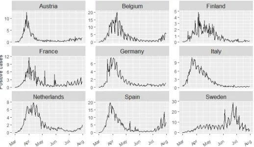
In Figure 1 we show the absolute number of reported infections per 100000 inhabitants. As for a very few days the reported number of positive cases are zero, we used time series imputation from the R package forecast [6] to replace the zeros by positive numbers. Most countries show a very similar pattern and reached their maximum number of cases around April; except for Sweden which reached it in June/July. We can see that some countries like Sweden, Spain and Belgium had much higher peaks. However, we can also see that the periods of high values around the peaks also differs a lot among the countries.
Figure 1. Number of reported COVID-19 infections per 100000 inhabitants from 2020-03-01 to 2020-07-31 for different countries.
To gain more insight into how one country performed in comparison to the whole group of countries we use the method described above. We estimate the multivariate trend filtering fits𝑎ˆ𝑡for𝑥𝑡, as described above, for𝜆chosen by𝐾= 10
fold cross validation and the one standard error rule, see Subsection 4.2, with 𝜆∈ {1,2,3,4,5,6,7,8,9,10,20,30}. In Figure 2, we plot the first pivot coordinate
√︁8 9log
(︂ (𝑥𝑡)𝑖
√8 ∏︀9
𝑗̸=𝑖(𝑥𝑡)𝑗
)︂
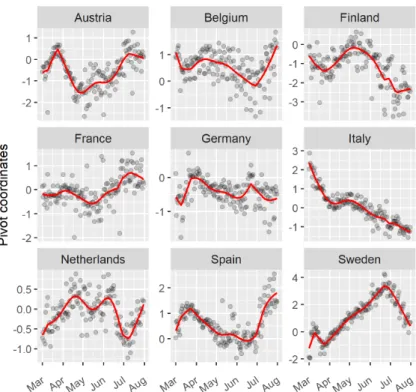
, where 𝑖 is the index corresponding to the 𝑖-th country in 𝑥𝑡, and the estimated trend. Pivot coordinates can be used to compare the fit (or number of cases) of one country to the geometric mean of the fit (or number of cases) of the rest of the group, containing all relative information of a specific part to the remaining parts in the considered composition [5].
Figure 2. Positive COVID-19 cases in first pivot coordinate per country. The black dots are the measured number of cases in the first pivot coordinate for each country. Equally, the red lines are its
compositional trend filtering fits for𝜆= 10.
It can be seen in Figure 2 that, compared to the whole group, Germany and Finland have had a comparatively low number of cases, as the values are mainly negative. Finland experienced a trend change in the middle/end of March with rising numbers compared to the geometric mean of the rest of the group, whereas Germany experienced a downward one. It is interesting to see that many coun- tries have had a change in trend since mid/end June - e.g. Belgium, Germany and Sweden. For instance, since the absolute numbers in Spain and Belgium have been rising quickly in July, more than in other countries, also a relative increase com-
pared to the other countries is visible. The contrary behaviour can be seen for Sweden, with a decay in relative number in the beginning of July. It is also sur- prising to see that Italy, which had the highest infection numbers at the beginning all over Europe, has constantly been improving compared to the other countries, and is by the end of June doing better than average. The Netherlands have at the end of July had average numbers however, its trend might have been alarming.
Furthermore, for a fixed country it might also be interesting to see how the trend of positive cases behaves compared to one other country. For this we display in Figure 3 the log-ratios of Austria and each country present in the composition.
Figure 3. Log-ratios of Austria and all other countries of the com- position. The black points are the observations, in red we display the compositional trends and in blue the regular univariate trend- filtering estimates. 𝜆was chosen in both cases by cross validation
with the one standard error rule.
We plot the compositional trend filtering fit described by the method above, which was also used for Figure 2, in log-ratios in red. Additionally, we show the univariate non-compositional trend filtering fits to each log-ratio pair in blue with𝜆obtained by cross validation with the one standard error rule as implemented in the R package [2]. We can see from the log-ratio between Austria and Germany that since July Austria has increasingly more cases than Germany. This upward trend has already started at the beginning of May when Austria still had less positive cases. At the same time the trend for the log-ratio between Austria and Italy started to change. This means that the positive cases per 100000 inhabitants in Austria is growing at a faster rate compared to each, Germany and Italy, since the beginning of July. Something similar holds for the pair Austria and Finland. At the end of July we can see that the cases in Austria compared to Italy or Finland
show a similar trend and numbers – around two. This is surprising as Italy notably started off with the highest infection numbers. At last, since July, Belgium and Spain seem do be doing worse and worse compared to Austria, indicated by a very steep downward trend. The non-compostional univariate trend filtering estimates (in blue) show a slightly different picture. The compositional approach differs sometimes vastly, e.g. for the log-ratio Austria-France, and seems to follow the data better where the non-compositional approach oversmooths, e.g. the log-ratio Austria-Spain in March, end of April and end of June. We also note that the compositional nature leads to trends which on the one hand are at times very smooth, and on the other, also display rapid changes.
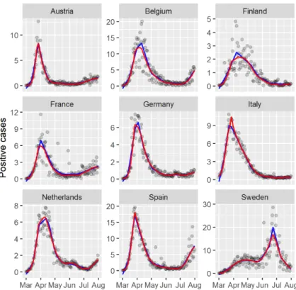
Figure 4. The black dots show for every country the recorded number of positive cases per 100000 inhabitants. The red lines dis- play the estimator𝑃𝑡𝑎^𝑡. The blue lines display the trends estimated
by non-compositional trend filtering.
The fit (ˆ𝑢1, . . . ,𝑢ˆ𝑇)′ can also be back-transformed to (ˆ𝑎1, . . . ,𝑎ˆ𝑇)′ into the simplex, and the elements per time point sum up to 1. If we want to present those back-transformed fits together with the absolute numbers of infections per 100000 inhabitants, we need to multiply with the total𝑃𝑡per time point. However, as we want to keep the smoothness of the fits, we will multiply with a smoothed total, as
described at the end of Section 3. To do this we sum up at each time point for all countries the number of positive cases, log-transform the latter and divide it by the absolute maximum, fit a smoother – in our case a univariate trend filter from the R package genlasso [2] with 𝜆= 1 – and transform it back by multiplying it first with the absolute maximum of the log-transform and then taking its exponential.
In Figure 4 we display the fit𝑃𝑡𝑎ˆ𝑡to the original points in red. In blue we show the univariate non-compositional trend filtering fits for𝜆= 1, where the data were first divided by the maximum, then the trend filtering fit was obtained, and lastly, the latter was again multiplied by the maximum. Dividing the data by the absolute maximum before fitting puts the𝜆on a similar footing for comparison with𝑃𝑡𝑎ˆ𝑡. Note that the estimator 𝑃𝑡𝑎ˆ𝑡 always sums up to the total 𝑃𝑡, as we are taking a compositional approach. It is interesting to see that for most countries the highest number of cases had been reached around mid/end of March with a change in trend since then. Also note that the fitted trend to Italy in the first half of April seems to be larger than one would expect from the data in Euclidean space. Examining the data at this time more closely we can see that the number of positive cases actually is very high for two consecutive days, before suddenly dropping and so the compostional fit reflects this better than the non-compositional one. Lastly, the non-compositional approach gives a negative estimate at the beginning of the measurements and shows a slightly different behaviour at the peaks.
6. Summary and conclusions
In this paper we presented a new method for fitting piecewise compositional linear trends to compositional time series. The method we proposed is a direct extension of univariate trend filtering to the compositional setting, which is multivariate by definition. This was done by reformulating the optimization problem in the appropriate Aitchison geometry on the simplex. We showed how to derive the problem in the usual Euclidean geometry, expressed in ilr coordinates, and that the solution does not depend on the specific choice of ilr coordinates. We proceeded by describing how to efficiently solve the problem through an ADMM algorithm.
To show the usefulness of our method, we looked at the number of COVID- 19 cases in different European countries in the period from March to July 2020.
Namely, once the compositional trend was fitted, we explored the trends in Pivot coordinates and log-ratio representations. This gave insights into how the COVID- 19 infections in some countries behaved compared to the compositional mean of other countries, during the said time period.
The fitted trends have been back-transformed to the simplex. The results have to sum up to 1 per time point, and the values cannot be negative – which is often a desirable property. After multiplication by a smoothed total for every country, the total infection numbers can be compared to the smooth line, which still represents relative information to all other countries, and deviations might indicate interesting phenomena (higher variability, etc.).
Additionally to the compositional time series case presented in this paper, one
could look at various extensions. For example, instead of looking at compositional data with a time stamp, one could also look at compositional data with a geographic stamp. That means that we would look at a random variable𝑥(𝑢,𝑠)∈ 𝒮𝐷−1 with (𝑢, 𝑠)being a geographic location. Such a case might be interesting for geochemical exploration where at certain geographic points we measure the concentration of elements. For the latter a shift in concentrations might correspond to interesting areas, thus leading to piecewise constant trend filtering in the compositional sense.
Another extension might consider robustification of the proposed method. Outliers are quite common in any statistical setting and compositional data are just as much affected by such. Therefore, investigating a compositionally robust definition of trend filtering might be interesting.
References
[1] J. Aitchison:The statistical analysis of compositional data, Journal of the Royal Statistical Society: Series B (Methodological) 44.2 (1982), pp. 139–160,
doi:https://doi.org/10.1111/j.2517-6161.1982.tb01195.x.
[2] T. B. Arnold,R. J. Tibshirani:Package ‘genlasso’, Statistics 39.3 (2020), pp. 1335–1371.
[3] S. Boyd,N. Parikh, E. Chu: Distributed optimization and statistical learning via the alternating direction method of multipliers, Now Publishers Inc, 2011,
doi:https://doi.org/10.1561/9781601984616.
[4] L. Breiman,J. Friedman,C. J. Stone,R. A. Olshen:Classification and Regression Trees, CRC Press, 1984.
[5] P. Filzmoser,K. Hron,M. Templ:Applied Compositional Data Analysis, Switzerland:
Springer Nature (2018),
doi:https://doi.org/10.1007/978-3-319-96422-5.
[6] R. Hyndman,G. Athanasopoulos,C. Bergmeir,G. Caceres,L. Chhay,M. O’Hara- Wild,F. Petropoulos,S. Razbash,E. Wang,F. Yasmeen:forecast: Forecasting func- tions for time series and linear models, R package version 8.13, 2020,
url:https://pkg.robjhyndman.com/forecast/.
[7] S. J. Kim,K. Koh,S. Boyd,D. Gorinevsky:𝑙1trend filtering, SIAM Review 51.2 (2009), pp. 339–360,
doi:https://doi.org/10.1137/070690274.
[8] N. Parikh, S. Boyd: Proximal algorithms, Foundations and trends in optimization 1.3 (2014), pp. 127–239,
doi:https://doi.org/10.1561/2400000003.
[9] A. Ramdas, R. J. Tibshirani: Fast and flexible ADMM algorithms for trend filtering, Journal of Computational and Graphical Statistics 25.3 (2016), pp. 839–858.
[10] V. Sadhanala, R. J. Tibshirani: Additive models with trend filtering, arXiv preprint arXiv:1702.05037 (2017).
[11] R. J. Tibshirani:Adaptive piecewise polynomial estimation via trend filtering, The Annals of Statistics 42.1 (2014), pp. 285–323,
doi:https://doi.org/10.1214/13-AOS1189.
[12] R. Tibshirani:Regression shrinkage and selection via the lasso, Journal of the Royal Sta- tistical Society: Series B (Methodological) 58.1 (1996), pp. 267–288,
doi:https://doi.org/10.1111/j.2517-6161.1996.tb02080.x.
[13] R. Varma,H. Lee,J. Kovačević,Y. Chi:Vector-valued graph trend filtering with non- convex penalties, IEEE Transactions on Signal and Information Processing over Networks 6 (2019), pp. 48–62,
doi:https://doi.org/10.1109/TSIPN.2019.2957717.
[14] B. Wahlberg,S. Boyd,M. Annergren,Y. Wang:An ADMM algorithm for a class of total variation regularized estimation problems, IFAC Proceedings Volumes 45.16 (2012), pp. 83–88,
doi:https://doi.org/10.3182/20120711-3-BE-2027.00310.
[15] Y.-X. Wang,J. Sharpnack,A. J. Smola,R. J. Tibshirani:Trend filtering on graphs, The Journal of Machine Learning Research 17.1 (2016), pp. 3651–3691.
[16] M. Yuan,Y. Lin:Model selection and estimation in regression with grouped variables, Journal of the Royal Statistical Society: Series B (Statistical Methodology) 68.1 (2006), pp. 49–67,
doi:https://doi.org/10.1111/j.1467-9868.2005.00532.x.