Decentralized Clearing in Financial Networks

Decentralized Clearing in Financial Networks

by Péter Csóka , P. Jean-Jacques Herings

C O R VI N U S E C O N O M IC S W O R K IN G P A PE R S

http://unipub.lib.uni-corvinus.hu/2508

CEWP 14 /201 6

Decentralized Clearing in Financial Networks ^∗

P´ eter Cs´ oka

P. Jean-Jacques Herings

November 3, 2016

Abstract

We consider a situation in which agents have mutual claims on each other, sum- marized in a liability matrix. Agents’ assets might be insufficient to satisfy their liabilities leading to defaults. In case of default, bankruptcy rules are used to specify the way agents are going to be rationed. A clearing payment matrix is a payment matrix consistent with the prevailing bankruptcy rules that satisfies limited liability and priority of creditors. Since clearing payment matrices and the corresponding values of equity are not uniquely determined, we provide bounds on the possible lev- els equity can take. Unlike the existing literature, which studies centralized clearing procedures, we introduce a large class of decentralized clearing processes. We show the convergence of any such process in finitely many iterations to the least clearing payment matrix. When the unit of account is sufficiently small, all decentralized clearing processes lead essentially to the same value of equity as a centralized clear- ing procedure. As a policy implication, it is not necessary to collect and process all the sensitive data of all the agents simultaneously and run a centralized clearing procedure.

Keywords: Networks, Bankruptcy Problems, Systemic Risk, Decentralized Clearing, Indivisibilities.

JEL Classification: C71, G10.

∗We would like to thank P´eter Bencz´ur, P´eter Bir´o, D´avid Csercsik, Mikl´os Pint´er, Adam Zawadowski and participants of East Asian Conference on Game Theory, Corvinus Game Theory Seminar, 6th Annual Financial Market Liquidity Conference and 10th Workshop on Economic Design and Institutions for helpful comments.

†Corvinus University of Budapest, Corvinus Business School, Department of Finance and “Momentum”

Game Theory Research Group, Centre for Economic and Regional Studies, Hungarian Academy of Sciences.

E-mail: peter.csoka@uni-corvinus.hu. P´eter Cs´oka thanks funding from National Research, Development and Innovation Office (NKFIH, PD 105859), from HAS (LP-004/2010) and from COST Action IC1205 on Computational Social Choice.

‡Department of Economics, Maastricht university, P.O. Box 616, 6200 MD, Maastricht, The Nether- lands. E-mail: P.Herings@maastrichtuniversity.nl.

1 Introduction

The treatment of bankruptcy of countries, banks, firms, organizations, and individuals will always be a challenge for society. In the original bankruptcy problem, starting with the seminal paper of O’Neill (1982), there is a single bankrupt agent and the other agents have claims on the estate of the bankrupt agent. In this paper, we analyze networks of agents, where agents have mutual claims on each other. An agent is characterized by his endowments and his liabilities towards the other agents. The assets of an agent consist of the sum of his endowments and the payments received from other agents having liabilities to him.

If the assets of an agent are not sufficient to satisfy his own liabilities, then the agent has to default. In a network setting, a default can also result from contagion, where an agent defaults only because other agents are not fully paying their liabilities to him. The default of a single agent can therefore result in domino effect that potentially leads to an all encompassing cascade of defaults. We are interested in the final resulting outcome in terms of payments and equity and in particular in the question whether one needs to use centralized clearing procedures as is assumed in the systemic risk literature, or whether one can rely on decentralized clearing processes as introduced in this paper instead.

An important application of our model concerns financial networks, where Eisenberg and Noe (2001) is the seminal paper. Recent crisis on financial markets triggered by the Lehman bankruptcy as well as sovereign debt problems of European countries provide prime examples of why the network perspective is important. Part of the literature on financial networks concerns the appropriate measurement of systemic risk, see Chen et al.

(2013) for an axiomatic approach as well as Demange (2015). There is also a substantial literature that relates the number and magnitude of defaults to the network topology and that characterizes those structures that tend to propagate default, see Gai and Kapadia (2010), Elliott et al. (2014), Acemoglu et al. (2015), Capponi et al. (2015), and Glasserman and Young (2015). The basic setup of Eisenberg and Noe (2001) has also been extended in various directions, for instance in Cifuentes et al. (2005) and Shin (2008) by allowing for liquidity considerations and in Rogers and Veraart (2013) by allowing for costs of default.

Given the prominence of the financial applications, we use the terminology of that framework, but want to emphasize that our model is relevant outside that specific setup.

Indeed, network effects of defaults occur also outside financial settings. Brown (1979) presents an application of a supply chain network consisting of coal mines and power companies, where due to a strike only the non-union mines produce and the other mines default on their deliveries of coal. Another example is related to international student exchange problems, as well as the closely related problem of tuition exchange studied in Dur and ¨Unver (2015), where the agents correspond to colleges. The endowments of a

college equal the maximum net inflow of students it can handle, its liabilities correspond to commitments made to receive incoming students, and claims are the agreements with other colleges to send outgoing students. As another example, the agents can be servers that process jobs for a set of users. The endowments of a server correspond to its capacity for processing jobs, its liabilities to jobs that it has to process for other servers, and its claims to jobs that are outsourced to other servers. An example similar to the one with servers concerns time banks, where the agents are workers instead of servers.

A clearing payment matrix describes how much the agents pay to each other. The lit- erature on financial networks has presented a number of algorithms to compute a clearing payment matrix and emphasize the computation of the greatest clearing payment ma- trix. Examples of such algorithms are presented in Eisenberg and Noe (2001), Rogers and Veraart (2013), and Elliott et al. (2014). These algorithms correspond to centralized pro- cedures for finding a clearing payment matrix. The required levels of payments during the execution of the algorithm are typically not implementable and are computed by solving a joint optimization program or a simultaneous system of equations.

As noted in Elsinger et al. (2006) and Gai and Kapadia (2010), the complexity of the financial system means that policymakers have only partial information about the true linkages between financial intermediaries. It is therefore not realistic to assume that a single decision maker has all the information that is needed for the execution of the algorithms.

On top of that, it is not realistic to assume that all assets of defaulting agents can be liquidated instantaneously.

Whereas the entire literature on systemic risk has considered centralized procedures to compute a clearing payment matrix, we introduce a large class of decentralized clearing processes in this paper. At each point in time, an agent is selected by means of a process that is potentially history-dependent and stochastic. This agent would typically be an agent that has filed for bankruptcy. Next, the selected agent makes any amount of feasible payments to the other agents. The amount that is paid depends only on local information and is determined by a process that again is potentially history-dependent and stochastic.

The only requirement that we make is that the selected agent be eligible, that is can make a positive incremental payment without ending up with negative equity.

To define the class of decentralized clearing processes, it is mathematically convenient to express all quantities in some smallest unit of account (dollars, number of students, number of jobs, etc.) and work in a discrete setup. We also show that our main result, on finite convergence of any decentralized clearing process in our class, is not true in the perfectly divisible case. The discrete setup has also been analyzed in the bankruptcy literature with multiple claimants on a single estate, see Young (1994) Moulin (2000), Moulin and Stong (2002), Herrero and Mart´ınez (2008), and Chen (2015), but so far not in a network setting

and the emphasis in that literature is on the axiomatic foundation of allocation rules. All papers in the systemic risk literature stick to the perfectly divisible approach.

We think of the discrete model as being more general than the perfectly divisible model.

On the one hand, using integers, we can study all the financial applications, where the unit of account can be taken to be one cent or one dollar and it is really a matter of mathematical convenience whether one uses a model with integers or reals. At the same time, we can study all the applications where indivisibilities matter like the mentioned applications of international student exchange or job processing by a network of servers, where realism dictates the use of integers rather than reals.

If an agent is bankrupt, then a bankruptcy rule specifies how the liabilities of vari- ous creditors are going to be settled. Following the seminal paper by Eisenberg and Noe (2001), the literature on systemic risk in financial networks has adopted proportional rules specifying payment ratios less than one in case of default. In reality, not all the liabilities are of the same seniority and some of the liabilities are more senior than others. American bankruptcy law, for instance, is a mixed lexicographic-proportional system, see Kaminski (2000). We therefore allow for general bankruptcy rules and present a convenient repre- sentation for them.

A clearing payment matrix is characterized by the properties of feasibility, limited liability, and priority of creditors. Feasibility of a payment matrix means that payments are made in accordance with bankruptcy rules. Limited liability means the payment matrix should result in non-negative equity levels for all agents. Priority of creditors requires that if an agent is not paying all of its liabilities, then a higher payment should lead to a negative equity level.

We characterize all clearing payment matrices as a fixed point of an appropriately de- fined function. We show that there exist a least and a greatest clearing payment matrix.

Unlike the perfectly divisible case, different clearing payment matrices may result in dif- ferent amounts of equity. We provide lower and upper bounds on the maximum difference in equity value that results from two different clearing payment matrices.

We show that any decentralized process in a large class converges in finitely many iterations to the least clearing payment matrix. In this sense, the cost of decentralization is therefore to go from the greatest to the least clearing payment matrix. The bounds we derive on the final levels of equity show that this cost is typically small in financial applications. Thus as a policy implication for financial applications, instead of working on collecting and processing data centrally, we suggest that it is sufficient to have local liquidators enforcing bankruptcy rules.

This paper is organized as follows. Section 2 presents the model of financial networks, the representation of bankruptcy rules, and some examples. Section 3 defines clearing

payment matrices. In Section 4 we analyze clearing payment matrices as fixed points and derive the bounds for the difference in equity value that results from two different clearing payment matrices. Section 5 introduces a large class of decentralized clearing processes and shows how any process in this class converges to the least clearing payment matrix in a finite number of iterations. Section 6 deals with the relationship between the discrete and the perfectly divisible case. Section 7 concludes.

2 Financial Networks

In the bankruptcy literature, there is typically a single bankrupt agent and the estate is an exogenously given amount.¹ The emphasis of the analysis is on the study of normative properties of different bankruptcy rules. The systemic risk literature invariably uses the proportional bankruptcy rule. In that literature there are multiple defaulting agents and the estates are endogenously determined. In this section, we develop our model of financial networks that combines insights from both literatures.

The primitives of a financial network are given by the tuple (z, L, b).

Let N0 denote the natural numbers including 0. The vector z ∈ N^I0 represents the endowments of the agents in the finite set of agents I with cardinality n. The endowment of an agent includes all his tangible and intangible assets, but excludes the claims and liabilities such an agent has towards the other agents. We work in the space of natural numbers, so implicitly it is assumed that everything is expressed in a smallest unit of account, which could be one dollar or one cent in the financial applications.

The n×nliability matrixL∈N^I×I0 describes the mutual claims of the agents. Its entry L_ij is the liability of agent itowards agent j or, equivalently, the claim of agent j on agent i. We make the normalizing assumption that L_ii= 0 for alli∈I. In general, it can occur that agent i has a liability towards agent j and agent j has a liability towards agent i, so bothL_ij >0 and L_ji >0 can occur simultaneously.

The payments to be made by agent i ∈ I to the other agents are determined by the bankruptcy ruleb_i :N0 →N^I0 of agenti. Given a valueE_i ∈N0 of the estate of agenti,the

1For surveys of the literature on bankruptcy problems, we refer the reader to Thomson (2003), Thom- son (2013), and Thomson (2015). There is also an emerging literature on the extension of the bankruptcy literature to network settings. The emphasis in these papers is on the axiomatic foundation of allocation rules. Bjørndal and J¨ornsten (2010) analyze generalized bankruptcy problems with multiple estates as flow sharing problems and define the nucleolus and the constrained egalitarian solution for such problems.

Moulin and Sethuraman (2013) consider bipartite rationing problems, where agents can have claims on a subset of unrelated estates. They consider whether rules for single resource problems can be consis- tently extended to their framework. Groote Schaarsberg et al. (2013) axiomatize the Aumann-Maschler bankruptcy rule in financial networks with general division rules.

monetary amount b_ij(E_i)∈N⁰ specifies how much agenti has to pay to agent j ∈I. The tuple (b_i)_i∈I of bankruptcy rules is denoted by b.

Contrary to the bankruptcy literature, the value of the estate E_i of agent i ∈ I is endogenously determined in a financial network, since it depends not only on the initial endowments of agent i, but also on the claims i has on other agents, part of which may not be received by agenti.Exactly how the value of the estate is endogenously determined is one of the important aspects studied in this paper and is addressed in the subsequent sections.

We make the following assumption on bankruptcy rules.

Assumption 1. Let (z, L, b) be a financial network. For everyi∈I, the bankruptcy rule b_i is a monotonic function b_i :N0 →N^I0 such that:

1. For every E_i ∈N0,P

j∈Ib_ij(E_i)≤min{P

j∈IL_ij, E_i} with equality if P

j∈IL_ij ≤E_i. 2. For every E_i ∈N0,for every j ∈I, b_ij(E_i)≤L_ij.

3. For every E_i, E_i⁰ ∈N0 such thatE_i ≤E_i⁰,P

j∈Ib_ij(E_i⁰)≤E_i impliesb_i(E_i) =b_i(E_i⁰).

Assumption 1 requires the bankruptcy rule b_i to be monotonic: For every E_i, E_i⁰ ∈ N0

such that E_i ≤ E_i⁰ it holds for every j ∈I that b_ij(E_i)≤b_ij(E_i⁰) or, equivalently,b_i(E_i)≤ b_i(E_i⁰). A weakly higher value of the estate leads to weakly higher payments to all agents.

This property is called resource monotonicity in the bankruptcy literature, see Thomson (2003), or endowment monotonicity, see Thomson (2015).

Assumption 1.1 allows for the possibility thatP

j∈Ib_ij(E_i)< E_i ifE_i <P

j∈IL_ij.Some of the estate may not be distributed among the agents in case the estate falls below the total value of the liabilities. We will illustrate how fairness considerations, like the fairness norm that equal claimants should receive an equal payment, can be at odds with the requirement thatP

j∈Ib_ij(E_i) =E_i wheneverE_i <P

j∈IL_ij.At the same time, we present several rules that do satisfy the requirement that P

j∈Ib_ij(E_i) = E_i whenever E_i < P

j∈IL_ij, so such rules are by no means excluded.

Assumption 1.2 specifies that a claimant never receives more than the value of his claim.

Assumption 1.3 puts limits on the extent to which paying less than the estate is possible.

If total payments made at the higher estate E_i⁰ do not exceed the value of the lower estate E_i, than those are also the payments made atE_i.

We continue by presenting a convenient representation for bankruptcy rules. The image F_i of a bankruptcy ruleb_i determines the set of feasible payments. More formally, we have

F_i =b_i(N0) = ∪_{{Ei∈N0|Ei≤}^P

j∈ILij}{b_i(E_i)},

where the second equality follows from the observation that by Assumptions 1.1 and 1.2 it holds that bi(Ei) = Li whenever Ei ≥ P

j∈ILij. The set of feasible payments Fi can

be found by considering the value of the bankruptcy rule for integer values of the estate between zero and the total amount of claims.

Assumption 1.3 corresponds to the requirement that bankruptcy rules impose maximal feasible payments. Indeed, b_i(E_i) is the maximal vector in F_i for which the sum of the components is less than or equal to E_i. Notice that the monotonicity of b_i implies that

≤ is a total order on the set F_i, i.e. the order ≤ on F_i is antisymmetric, transitive, and complete. A maximal vector in Fi for which the sum of the components is less than or equal to Ei is therefore uniquely determined.

Vice versa, any setTi ⊂N^I0,which is totally ordered by≤, contains 0^I,and has Li as a maximum, pins down a bankruptcy rule b^T_iⁱ with set of feasible payments equal toTi. For Ei ∈N⁰, let

b^T_iⁱ(E_i) = max{f_i ∈T_i |P

j∈If_ij ≤E_i}, (1)

where the maximum in (1) is unique sinceT_i is a finite set,T_i contains 0^I, and≤is a total order on T_i.The following proposition states that b^T_iⁱ indeed satisfies Assumption 1.

Proposition 1. For every i ∈ I, let T_i be a subset of N^I0, which is totally ordered by ≤, contains 0^I, and with maxT_i = L_i. Then the tuple of induced bankruptcy rules (b^T_iⁱ)_i∈I satisfies Assumption 1.

Proof. Let somei∈I be given. Clearly, it holds thatb^T_iⁱ is a monotonic function from N0 into N^I0.

If P

j∈IL_ij ≤E_i, then

b^T_iⁱ(E_i) = max{f_i ∈T_i |P

j∈If_ij ≤E_i}=L_i, where the second equality follows sinceP

j∈IL_ij ≤E_i.In this case, we therefore have that P

j∈Ib^T_ijⁱ(E_i) = min{P

j∈IL_ij, E_i}.

If P

j∈IL_ij > E_i, then P

j∈Ib^T_ijⁱ(Ei)≤Ei = min{P

j∈ILij, Ei},

where the inequality follows immediately from the definition of b^T_iⁱ(E_i). Assumption 1.1 is therefore satisfied.

Since T_i is totally ordered by ≤, we have, for every f_i ∈ T_i, f_i ≤ maxT_i = L_i. It now follows that, for every E_i ∈ N0, for every j ∈ I, b^T_ijⁱ(E) ≤ L_ij. This shows that Assumption 1.2 holds.

Let E_i, E_i⁰ ∈N0 be such thatE_i ≤E_i⁰ and P

j∈Ib^T_ijⁱ(E_i⁰)≤E_i. Since b^T_iⁱ(E_i⁰) = max{fi ∈Ti |P

j∈Ifij ≤E_i⁰}

and P

j∈Ib^T_ijⁱ(E_i⁰)≤E_i, it follows that b^T_iⁱ(E_i) = max{f_i ∈T_i |P

j∈If_ij ≤E_i}=b^T_iⁱ(E_i⁰).

We have shown that Assumption 1.3 holds. 2

An important class of bankruptcy rules consists of the priority bankruptcy rules. They depend on a permutation π : I → {1, . . . , n}, which indicates the rank of the various liabilities. Forj ∈I, we define

π^j ={i∈I |π(i)< π(j)}

as the set of agents ranked before agent j according to π.

Definition 1. Given a vector of liabilities Li ∈ N^I0 of agent i ∈ I and a permutation π :I → {1, . . . , n}, the priority bankruptcy rule b^π_i :N⁰ →N^I0 is defined by

b^π_ij(E_i) = max{0,min{L_ij, E_i−X

k∈π^j

L_ik}}, j ∈I, E_i ∈N0.

Under the bankruptcy rule b^π_i, the estate of agent i has a priority list of creditors as determined by the permutation π. The claims of agents π⁻¹(1), π⁻¹(2), . . . are paid for sequentially as long as the estate of agent i permits this.

A priority bankruptcy rule clearly satisfies Assumption 1. It also has the property that P

j∈Ib_ij(E_i) = min{E_i,P

j∈IL_ij} for every E_i ∈ N⁰, so the equality also holds in case P

j∈IL_ij > E_i. Priority bankruptcy rules have nice axiomatic foundations. As has been demonstrated in Moulin (2000) these are the only rules satisfying consistency, upper composition, and lower composition.²

Another frequently used bankruptcy rule is the proportional bankruptcy rule. It is easily defined when the estate and the payments are treated as real numbers. Given a vector of liabilities L_i ∈R^I0, the function d^prop_i :R⁺→R^I+ is defined by

d^prop_ij (E_i) = min{L_ij,^PLij

k∈IL_ikE_i}, j ∈I, E_i ∈R+.

2Consistency imposes that in case an agent leaves with the payment as described by the bankruptcy rule, then applying the bankruptcy rule to the smaller problem does not change the payments of the remaining agents. Upper composition requires that first applying the bankruptcy rule using a too optimistic value of the estate and using the resulting payments as the liabilities for the correct value of the estate leads to the same payments as directly applying the bankruptcy rule to the correct value of the estate. Lower composition is the dual of upper composition. It requires that first applying the bankruptcy rule using a too pessimistic value of the estate, revising the liabilities accordingly, and then dividing the remainder of the estate leads to the same result as directly applying the bankruptcy rule to the correct value of the estate.

Under the functiond^prop_ij ,the estate is divided in proportion to the liabilities. If the estate exceeds the sum of the liabilities, then every claimant receives his claim.³

The function d^prop_ij may not lead to integers, even if the estate is an integer. It is for this reason that Moulin (2000) describes the priority rules as the most natural rationing methods in the discrete model.

There are many ways to define a proportional rule while taking the integer require- ments into account. We present two such constructions here leading to the fair propor- tional bankruptcy rule and the quota bankruptcy rule, respectively. The fair proportional bankruptcy rule is based on the fairness principle that agents with equal claims should receive equal payments.

Given a set X ⊂R^I+,we define

bXc={f ∈N^I0 | ∃x∈X such thatf =bxc},

wherebxc denotes the vector obtained by taking for every i∈I the floor of x_i,the largest integer which is less than or equal to x_i.

Definition 2. Given a vector of liabilities L_i ∈ N^I0 of agent i ∈ I, the fair proportional bankruptcy rule b^prop_i :N0 →N^I0 is defined by

b^prop_i =b^bd

prop i (R+)c

i .

Under the fair proportional bankruptcy rule, all possible real-valued payment vectors d^prop_i (R⁺) are first rounded down to obtain the set of feasible payments Ti =bd^prop_i (R⁺)c.

Next, the fair proportional bankruptcy rule b^prop_i is defined by setting it equal to the bankruptcy rule b^T_iⁱ induced by T_i. Clearly, b^prop_i satisfies the fairness criterion that equal claimants receive an equal payment.

It is easily verified that bd^prop_i (R+)c satisfies the conditions of Proposition 1, so b^prop_i satisfies Assumption 1.

We illustrate the definitions of bankruptcy rule and set of feasible payments in the following example.

Example 1. We have three agentsI ={1,2,3}. Agent 1 has an initial endowmentz1 = 1 and his liabilities areL1 = (0,2,2) as presented in Table 1. We assume that agents 2 and 3 have no liabilities, so the estate of agent 1 is equal to his initial endowment, E1 =z1 = 1.

The network aspect is not relevant for this example and the only problem is therefore to divide the estate of agent 1.

First, let us consider priority bankruptcy rules, where priorities are described by the identity, π(1) = 1, π(2) = 2,and π(3) = 3,so first payments to agent 1 should be made, a

3The perfectly divisible case is treated in detail in Section 6.

E₁ L₁

1 0 2 2

Table 1: The estate and claims on the estate of agent 1 in Example 1.

possible remainder of the estate to agent 2, and if there is still part of the estate remaining, payments can be made to agent 3. Since agent 1 has no liability towards himself, it is easily verified that the set of feasible payments is given by

F₁ ={(0,0,0),(0,1,0),(0,2,0),(0,2,1),(0,2,2)}.

It therefore holds that b^π₁(1) = (0,1,0), so the entire estate goes to agent 2.

Second, let us consider the fair proportional bankruptcy rule. In this case we have F₁ =bd^prop₁ (R+)c={(0,0,0),(0,1,1),(0,2,2)}.

It follows that b^prop₁ (1) = (0,0,0), so no payments are made to any agent in this case.

Another possibility in defining the proportional rule is to emphasize efficiency rather than fairness and require that the entire estate be divided. In a different guise, that prob- lem has been extensively studied in the rich political science literature on apportionment.

Apportionment addresses how to allocate a fixed number of seats among regions according to their respective numbers of inhabitants as well as the related problem of how to allocate a fixed number of seats among political parties according to their respective votes. In bankruptcy problems, the estate E_i plays the role of the fixed number of seats, the agents in the set I correspond to either regions or the political parties, and the liability L_ij to either the number of inhabitants of region j or the number of votes of political party j.

Balinski and Young (1975) give an overview of many methods for apportionment that are used in practise, like the Jefferson method (known in the United states as the method of greatest divisors and in Europe as the method of d’Hondt), the Hamilton method (generally known as the Vinton method), the Webster method (known as the method of major frac- tions), and the Huntington method (known as the method of equal proportions). Balinski and Young (1975) make a new proposal themselves, called the quota method. Not all these methods qualify as bankruptcy rules. For instance, the Alabama paradox refers to the fact that the Hamilton method violates monotonicity, a property called house monotonicity in the apportionment literature.

The quota method of Balinski and Young (1975) is actually not a single solution but rather a set of solutions. One solution in the set is defined next and we call it the quota bankruptcy rule. To define it, we need some additional notation. Given a permutation π : I → {1, . . . , n}, the unique argument that has the highest priority according to π

among the arguments that maximize a function g defined on a subset K of I is denoted by arg max^π_k∈Kg(k), so if j ∈ arg max_k∈Kg(k) and for every i ∈ arg max_k∈Kg(k) it holds that π(j)≤π(i),then arg max^π_k∈Kg(k) = j.

Let some agent i ∈ I with liabilities L_i and estate E_i < P

j∈IL_ij be given and sup- pose agent i makes a payment P_i ∈ N^I0. The set of agents whose payment is below their proportional share is defined as

B_i(P_i, E_i) = {j ∈I |P_ij < ^PLij

k∈ILikE_i}.

Definition 3. Given a vector of liabilities L_i ∈ N^I0 of agent i ∈ I and a permutation π : I → {1, . . . , n}, the quota bankruptcy rule q_i^π : N0 → N^I0 is recursively defined as follows.

q^π_i(0) = 0^I. If 0< Ei <P

j∈ILij, then q^π_ij(E_i) =

( q^π_ij(Ei−1) + 1, if j = arg max^π_k∈B

i(q^π_i(Ei−1),E_i) Lik

q^π_ik(Ei−1)+1, q^π_ij(E_i−1), otherwise.

If E_i ≥P

j∈IL_ij, then q^π_i(Ei) =Li.

The quota bankruptcy rule is defined recursively for increasing values of the estate.

Given some value of the estate E_i, it considers the agents j⁰ in the set B_i(q_i^π(E_i−1), E_i) whose paymentq_ij^π0(E_i−1) at estateE_i−1 is strictly below theirquota(L_ij⁰/(P

k∈IL_ik))E_i at estateE_i.Among those agents, it considers the agentsk with the highest ratio of liability to payment when the payment would be increased by one,L_ik/(q_ik^π(E_i−1) + 1),and selects the agent with the highest priority according toπ to receive the additional unit. It follows from the results in Balinski and Young (1975) that the quota bankruptcy rule is monotonic.

It is clear that the quota bankruptcy rule always divides the entire estate when the total liabilities exceed the estate. It is now easily verified that quota bankruptcy rules satisfy Assumption 1. An interesting property of the quota bankruptcy rule is that it satisfies

b^PLij

k∈IL_ikE_ic ≤q_ij^π(E_i)≤ d^{P Lij}

k∈IL_ikE_ie,

so the payment received by every agent is always in between his quota when rounded down and his quota when rounded up.

Example 2. We consider again the primitives of Example 1, now assuming that the estate of agent 1 is subject to the quota bankruptcy rule. As before, priorities are described by the identity, π(1) = 1, π(2) = 2, and π(3) = 3. It is easily derived that

F1 ={(0,0,0),(0,1,0),(0,1,1),(0,2,1),(0,2,2)}.

It therefore holds thatq^π₁(1) = (0,1,0),so the entire estate goes to agent 2. While efficient, the quota bankruptcy rule is not fair. Agents 2 and 3 have identical claims on the estate of agent 1, but receive different payments.

Example 3. As a final example, consider the all-or-nothing bankruptcy rule, in which either all or none of the claims are being paid. An example of such a rule can be found in Acemoglu et al. (2015) who study banking networks and assume that banks are forced to liquidate their projects in full, e.g. because it is difficult to liquidate a fraction of an ongoing real project. Other examples would arise in applications with supply chain networks, where either a complete or no delivery takes place.

In Example 1, the set of feasible payments corresponding to the all-or-nothing bankruptcy rule is given by

F₁ = {(0,0,0),(0,2,2)}.

Using Proposition 1, it is easily shown that all-or-nothing bankruptcy rules satisfy As- sumption 1.

3 Clearing Payment Matrices

Let some financial network (z, L, b) be given. Ann×n payment matrix P ∈N^I×I0 collects the mutual payments of the agents, that is, Pij is the amount paid by agent i to agent j.

We make the normalizing assumption that Pii = 0 for all i ∈ I. The set of all payment matrices with this property is denoted by M.The partial order ≤on Mis defined in the usual way: ForP, P⁰ ∈ M,it holds thatP ≤P⁰ if and only ifPij ≤P_ij⁰ for all (i, j)∈I×I.

A payment matrix P ∈ M is feasible if for every i ∈ I it holds that Pi ∈ Fi, so a payment matrix is feasible if every row i of the matrix belongs to the set of feasible payments of agent i, that is payments are made in accordance with bankruptcy rules.

The set of all feasible payment matrices is denoted by P,so P ={P ∈ M | ∀i∈I, Pi ∈Fi}.

The sum of the initial endowments of an agent and the payments received from the other agents determines an agent’s asset value, more formally defined as follows.

Definition 4. Given a financial network (z, L, b) and a payment matrix P ∈ M,the asset value a_i(P) of agent i∈I is given by

a_i(P) =z_i+X

j∈I

P_ji.

The asset value of an agent will play the role of the estate E_i.

Subtracting the payments as made by an agent from his asset value yields an agent’s equity. More formally, we have the following definition.

Definition 5. Given a financial network (z, L, b) and a payment matrixP ∈ M, theequity e_i(P) of agent i∈I is given by

e_i(P) =a_i(P)−X

j∈I

P_ij =z_i+X

j∈I

(P_ji−P_ij). (2)

If agent i∈I has negative equity even when all agents pay all their liabilities, so if e_i(L) =z_i +X

j∈I

(L_ji−L_ij)<0,

then agentihas so-calledfundamental default. When an agent defaults only because other agents are not fully paying their liabilities to him, then the agent is said to have contagion default.

It holds that X

i∈I

e_i(P) =X

i∈I

z_i+X

i∈I

X

j∈I

(P_ji−P_ij) =X

i∈I

z_i. (3)

Payment matrices only lead to a redistribution of initial endowments.

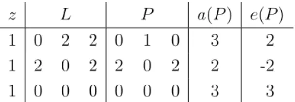
Example 4. Consider a financial network (z, L, b) with three agents I = {1,2,3} and endowments and liabilities as presented in Table 2. For everyi∈I,the bankruptcy ruleb_i equals the priority bankruptcy rule b^π whereπ is the identity, so agent 1 has priority over agent 2, who in turn has priority over agent 3.

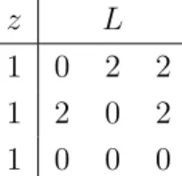
z L

1 0 2 2

1 2 0 2

1 0 0 0

Table 2: The endowments and liabilities of the agents in Example 4.

The payment matrix P in Table 3 is feasible since each row i is selected from the set of feasible payments F_i. Agent 1 has equity e₁(P) = 2, but still has unpaid liabilities to both agents 2 and 3. Agent 2 has negative equity, e₂(P) = −2. The payment matrix P suffers from two undesirable features. Agent 1 has a positive equity value and outstanding liabilities. Agent 2 has a negative equity value.

z L P a(P) e(P)

1 0 2 2 0 1 0 3 2

1 2 0 2 2 0 2 2 -2

1 0 0 0 0 0 0 3 3

Table 3: An undesirable payment matrix in Example 4.

To overcome this situation, we extend the notions of priority of creditors and limited liability defined in the perfectly divisible case for proportional rules by Eisenberg and Noe (2001) to our discrete setup with general bankruptcy rules.⁴

Definition 6. Given a financial network (z, L, b), P ∈ Mis a clearing payment matrix if it satisfies the following three properties:

1. Feasibility: P ∈ P.

2. Limited liability: For every i∈I, e_i(P)≥0.

3. Priority of creditors: For every i ∈ I, for every P_i⁰ ∈ F_i such that P_i⁰ > P_i it holds that a_i(P)−P

j∈IP_ij⁰ <0.

A clearing payment matrix is feasible, leads to non-negative equity values, and satisfies priority of creditors. Notice that priority of creditors is satisfied whenever P_i = L_i since there is no P_i⁰ ∈F_i with P_i⁰ > P_i in that case.⁵

The following proposition shows that in case the asset value of an agent is sufficient to pay all his liabilities, then the agent will do so in a clearing payment matrix.

Proposition 2. Let P be a clearing payment matrix for the financial network(z, L, b).For every i∈I, if a_i(P)≥P

j∈IL_ij, then P_i =L_i.

Proof. Suppose not. Let i∈I be such that a_i(P)≥P

j∈IL_ij and P_i < L_i. We define P_i⁰ =L_i,which is an element of F_i by Assumption 1. It holds that

a_i(P)−X

j∈I

P_ij⁰ =a_i(P)−X

j∈I

L_ij ≥0,

4Eisenberg and Noe (2001) refers to ‘priority of creditors’ as ‘priority of debt claims’ or ‘absolute priority’ and to ‘limited liability’ as ‘limited liability (of equity)’.

5In the perfectly divisible setup, priority of creditors is defined as follows by Eisenberg and Noe (2001):

For every i ∈ I, if Pi < Li, then ei(P) = 0. In the presence of integer payments, this condition is too strong. We therefore use the requirement in Condition 3 of Definition 6 that agentiends up with negative equity if he chooses a feasible payment that is strictly higher, whereas all other agents remain paying the same.

so P violates priority of creditors and is therefore not a clearing payment matrix, a con-

tradiction. 2

For the perfectly divisible setup with proportional rules, Eisenberg and Noe (2001) show that when all endowments are positive, then there is a unique clearing payment matrix.

Although in general multiple clearing payment matrices can co-exist, Eisenberg and Noe (2001) show that the final value of equity is the same irrespective of the clearing matrix that is being used. Glasserman and Young (2015) present other conditions to get a unique clearing payment matrix. For the perfectly divisible setup with general bankruptcy rules, though not allowing for agent specific bankruptcy rules, uniqueness of final equity values is shown in Groote Schaarsberg et al. (2013).

The next example shows that in the case with indivisibilities, the clearing payment matrix with fair proportional bankruptcy rules may not be unique even when all initial en- dowments are positive. More importantly, the resulting values of equity might be different as well.

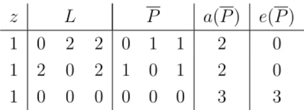
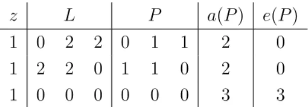
Example 5. As in Example 4, we consider a financial network (z, L, b) with three agents I ={1,2,3}and endowments and liabilities as presented in Table 2, but replace the priority bankruptcy rules of that example by fair proportional bankruptcy rules.

Table 4 presents the clearing payment matrix P and Table 5 the clearing payment matrix P . There are no other clearing payment matrices. The matrices P and P induce different equity values, e(P) = (1,1,1) ande(P) = (0,0,3).

z L P a(P) e(P)

1 0 2 2 0 0 0 1 1

1 2 0 2 0 0 0 1 1

1 0 0 0 0 0 0 1 1

Table 4: The clearing payment matrixP in Example 5, fair proportional bankruptcy rules.

z L P a(P) e(P)

1 0 2 2 0 1 1 2 0

1 2 0 2 1 0 1 2 0

1 0 0 0 0 0 0 3 3

Table 5: The clearing payment matrixP in Example 5, fair proportional bankruptcy rules.

It holds that e1(P) = e2(P) = 1, so there is some equity left for both agents 1 and 2 when the payment matrixP is used. Nevertheless, Condition 3 of Definition 6, priority of

creditors, holds since there is no higher feasible payment compatible with the asset values of agents 1 and 2.

Although Example 5 shows the possibility of multiple values of equity, the next section puts bounds on the maximum differences that are possible. For financial applications it will turn out that the consequences of having multiple equity values are not very serious.

On the other hand, if the application concerns a student exchange network, then some college not accepting a couple of students may trigger many other colleges doing the same, and in this case there could be significant effects.

4 Clearing Payment Matrices as Fixed Points

In this section, we characterize a clearing payment matrix as a fixed point of an appropri- ately defined function and derive the bounds for the difference between the values of equity for a given agent in any two clearing payment matrices.

Given a financial network (z, L, b),let ϕ:P → P be defined by ϕ_ij(P) =b_ij(a_i(P)), P ∈ P, i, j ∈I.

Proposition 3. Let a financial network (z, L, b) be given. The matrix P ∈ P is a clearing payment matrix if and only if P =ϕ(P).

Proof.

(⇒)

Consider some i∈I.We defineP_i⁰ =ϕ_i(P).Since P_i ∈F_i and b_i is monotonic, it holds that either (a) P_i < P_i⁰, or (b) P_i =P_i⁰, or (c) P_i > P_i⁰.

Case (a). P_i < P_i⁰. We have that

a_i(P)−X

j∈I

P_ij⁰ =a_i(P)−X

j∈I

ϕ_ij(P) =a_i(P)−X

j∈I

b_ij(a_i(P))≥0.

This contradicts the fact that P satisfies priority of creditors. We conclude that Case (a) cannot occur.

Case (c). P_i > P_i⁰.

Since P satisfies limited liability, it holds that e_i(P) ≥ 0. Let E_i ∈ N0 be such that P_i =b_i(E_i). From b_i(E_i) = P_i > P_i⁰ =b_i(a_i(P)), it follows that a_i(P)< E_i. Together with the fact that

X

j∈I

b_ij(E_i) =X

j∈I

P_ij =a_i(P)−e_i(P)≤a_i(P),

this implies by Assumption 1 thatb_i(a_i(P)) = b_i(E_i) and therefore thatP_i⁰ =P_i,a contra- diction to P_i > P_i⁰. We conclude that Case (c) cannot occur.

It now follows that Case (b) holds, so P_i =P_i⁰ =ϕ_i(P).

(⇐)

1. Feasibility. It holds that P ∈ P by the definition of ϕ.

2. Limited liability. For every i∈I, we have that Pi =ϕi(P) = bi(ai(P)),

so

ei(P) =ai(P)−X

j∈I

Pij =ai(P)−X

j∈I

bij(ai(P))≥ai(P)−ai(P) = 0.

3. Priority of creditors. Let i ∈ I and P_i⁰ ∈ F_i be such that P_i⁰ > P_i. Let E_i⁰ ∈ N⁰ be such that b_i(E_i⁰) =P_i⁰.Since b_i(a_i(P)) =P_i < P_i⁰ =b_i(E_i⁰), monotonicity ofb_i implies that E_i⁰ > a_i(P).

Suppose, by contradiction, that a_i(P)−P

j∈IP_ij⁰ ≥0. Then it holds that X

j∈I

b_ij(E_i⁰) = X

j∈I

P_ij⁰ ≤a_i(P).

Since E_i⁰ > ai(P), it follows from Assumption 1 that Pi =bi(ai(P)) =bi(E_i⁰).

We conclude thatPi =P_i⁰, a contradiction to the assumption that P_i⁰ > Pi. 2 A lattice is a partially ordered set in which every pair of elements has a supremum and an infimum. A complete lattice is a lattice in which every non-empty subset has a supremum and an infimum. Any finite lattice can be shown to be complete. The infimum of a two-point set {x, x⁰} is denoted byx∧x⁰ and its supremum by x∨x⁰.

The matrices in P are partially ordered by ≤, since ≤ is a reflexive, transitive, and antisymmetric order onP.

Consider two matrices P, P⁰ ∈ P.We define the matrices P , P ∈ P by P_i = P_i∧P_i⁰, i∈I,

P_i = P_i∨P_i⁰, i∈I.

Since Fi is totally ordered by ≤, it holds that P_i is either equal to Pi or to P_i⁰. Similarly, it holds thatPi is either equal toPi or to P_i⁰. It is now immediate thatP , P ∈ P and that P ∧P⁰ =P and P ∨P⁰ =P . Every pair of matrices in P therefore has a supremum and an infimum in P.We conclude that the set P is a complete lattice.

Proposition 4. Consider a financial network (z, L, b). The set of clearing payment ma- trices is a complete lattice. In particular, there exists a least clearing payment matrix P⁻ and a greatest clearing payment matrix P⁺.

Proof. We show that ϕ is monotone. Let P, P⁰ ∈ P be such that P ≤ P⁰. For every i∈I, it holds that

ϕ_i(P) = b_i(a_i(P)) =b_i(z_i+X

j∈I

P_ji)≤b_i(z_i+X

j∈I

P_ji⁰) = b_i(a_i(P⁰)) = ϕ_i(P⁰),

where the inequality follows from the monotonicity of b_i.

By Tarski’s fixed point theorem (Tarski, 1955), the set of fixed points ofϕis a complete lattice with respect to ≤. It follows that the set of fixed points has a least and a greatest element. By Proposition 3, the set of fixed points of ϕ is equal to the set of clearing pay-

ment matrices. 2

Example 5 shows that two clearing payment matrices may lead to different values of equity. To analyze the size of the possible differences, we introduce the following notation.

For every i∈I,for everyP_i ∈F_i\ {L_i},we define S_i(P_i) as the unique successor ofP_i,i.e.

the lowest feasible payment vector that is strictly greater than P_i. Note that S_i(P_i) is not defined if P_i =L_i.

For every i∈ I, the number κ_i equals the maximal difference between total payments in two consecutive feasible payment vectors for agent i. If F_i consists of a single element, so F_i = {L_i} ={0^I}, then we define κ_i = 1. Otherwise, F_i has at least two elements and we define

κ_i = max

Pi∈Fi\{Li}

X

j∈I

(S_ij(P_i)−P_ij).

The bankruptcy rules discussed in Section 2 give three typical numbers forκ_i.Ifb_i is a pri- ority bankruptcy rule or a quota bankruptcy rule, thenκ_i = 1.Ifb_i is the fair proportional bankruptcy rule andL_i >0,thenκ_i is at most as large as the number of non-zero liabilities λ_i = #{j ∈I |L_ij >0} of agent i,which in turn is less than the number of agents n. Ifb_i corresponds to the all-or-nothing bankruptcy rule and L_i >0, then κ_i = P

j∈IL_ij equals the sum of the liabilities of agent i.

The numbers κ_i for i∈I can be used to provide lower and upper bounds on the maxi- mum difference in equity value that results from two different clearing payment matrices.

Proposition 5. Consider a financial network (z, L, b) and two clearing payment matrices P andP⁰ withP ≤P⁰. For every i∈I,the difference between the value of equity at P and P⁰ satisfies −(κ_i−1)≤e_i(P⁰)−e_i(P)≤P

j∈I\{i}(κ_j−1).

Proof. We argue first that, for every i∈I, max{0, a_i(P)−P

j∈IL_ij}=a_i(P)−P

j∈IP_ij −ε_i(P) =e_i(P)−ε_i(P), (4) where

ε_i(P)∈







{0}, if ai(P)≥P

j∈ILij, {0, . . . , κ_i−1}, if a_i(P)<P

j∈IL_ij. We distinguish two cases: (a) a_i(P)≥P

j∈IL_ij and (b) a_i(P)<P

j∈IL_ij. Case (a). a_i(P)≥P

j∈IL_ij. It holds that

max{0, a_i(P)−P

j∈IL_ij}=a_i(P)−P

j∈IL_ij =a_i(P)−P

j∈IP_ij =e_i(P), where the second equality follows from Proposition 2. It follows that ε_i(P) = 0.

Case (b). a_i(P)<P

j∈IL_ij. It holds that

εi(P) =ei(P)−max{0, ai(P)−P

j∈ILij}=ei(P). (5)

Since P is a clearing payment matrix, it follows that ε_i(P) ∈ N⁰. Moreover, we have by Proposition 3 that

P

j∈IP_ij =P

j∈Ib_ij(a_i(P))≤min{P

j∈IL_ij, a_i(P)}=a_i(P)<P

j∈NL_ij. Since P satisfies priority of creditors, we have that

a_i(P)−X

j∈I

S_ij(P_i)<0.

Finally, using Equation (5), it follows that ε_i(P) =e_i(P) =a_i(P)−X

j∈I

P_ij ≤a_i(P)−X

j∈I

S_ij(P_i) +κ_i ≤κ_i−1.

This completes the proof that Equation (4) holds.

Let some i∈I be given. SinceP ≤P⁰, we have that max{0, a_i(P)−P

j∈IL_ij} ≤max{0, a_i(P⁰)−P

j∈IL_ij}, so it follows from Equation (4) that

ei(P)−εi(P)≤ei(P⁰)−εi(P⁰).

Rewriting this inequality, we obtain

e_i(P⁰)−e_i(P)≥ε_i(P⁰)−ε_i(P)≥ −(κ_i −1).

Using Equation (3), we find that e_i(P⁰)−e_i(P) = X

j∈I\{i}

(e_j(P)−e_j(P⁰))≤ X

j∈I\{i}

(κ_j −1),

which completes the proof. 2

By Proposition 4, it holds for any clearing payment matrix P that P⁻ ≤ P ≤ P⁺. Natural choices in Proposition 5 are thereforeP =P⁻ and P⁰ =P⁺.

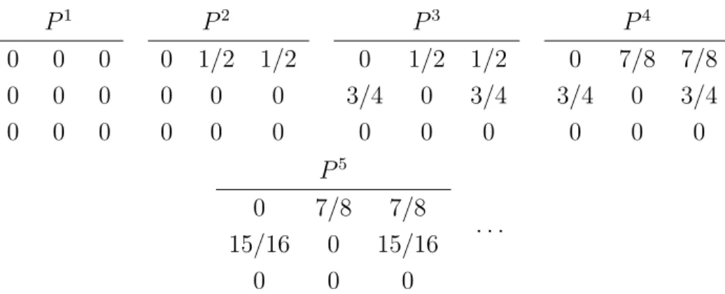
In Example 5 it holds that κ₁ = κ₂ = 2 and κ₃ = 1. There are only two possible clearing payment matrices, P and P .It holds that e₁(P)−e₁(P) =e₂(P)−e₂(P) =−1 =

−(κ₁−1) =−(κ₂−1), so the lower bound of Proposition 5 is tight. Sincee₃(P)−e₃(P) = 2 = (κ₁−1) + (κ₂−1), the upper bound of Proposition 5 is tight as well.

In a financial network with priority or quota bankruptcy rules, or more generally, in a financial network where κ_i = 1 for every i ∈ I, Proposition 5 implies that the difference between the value of equity for a given agent at the least clearing payment matrix P⁻ and any clearing payment matrixP is zero. The value of equity is uniquely determined in this case.

In a financial network with fair proportional bankruptcy rules, the difference between the value of equity of agentiat the greatest clearing payment matrixP⁺ and any clearing payment matrix P is bounded between −λ_i ≥ −(n −1) and P

j∈I\{i}(λ_j − 1) ≤ (n − 1)(n−1−1) = (n−1)(n−2) by Proposition 5. If all bankruptcy rules are all-or-nothing, then this difference is bounded between −(κ_i −1) ≥ −P

j∈IL_ij and P

j∈I\{i}(κ_j −1) ≤ P

j∈I\{i}

P

k∈IL_jk.

5 Decentralized Clearing

The literature on default in financial networks has so far always considered centralized clearing procedures. In this section, we introduce a large class of decentralized clearing processes. We show that any process in this class converges to the least clearing payment matrix. Bounds on equity differences with the greatest clearing payment matrix are given by Proposition 5.

In a centralized clearing procedure, implicitly all agents are filing for bankruptcy si- multaneously and a clearing payment matrix is centrally computed. One possibility to do so is by formulating an integer programming problem where the objective is to maximize