Why APRC is misleading and how it should be reformed
by Edina Berlinger
C O R VI N U S E C O N O M IC S W O R K IN G P A PE R S
http://unipub.lib.uni-corvinus.hu/3040
CEWP 5 /201 7
1
Why APRC is misleading and how it should be reformed
Edina Berlinger1
Department of Finance, Corvinus University of Budapest 10.09.2017
Abstract
The annual percentage rate of charge (APRC) designed to reflect all costs of borrowing is a widely used measure to compare different credit products. It disregards completely, however, risks of possible future changes in interest and exchange rates. As an unintended consequence of the general advice to minimize APRC, many borrowers take adjustable-rate mortgages with extremely short interest rate period or foreign currency denominated loans and run into an excessive risk without really being aware of it. To avoid this, we propose a new, risk- adjusted APRC incorporating also the potential costs of risk hedging. This new measure eliminates most of the virtual advantages of riskier structures and reduces the danger of excessive risk taking. As an illustration, we present the latest Hungarian home loan trends but lessons are universal.
JEL-codes: G18, G21, G28, G41
Keywords: mortgage lending, annual percentage rate of charge, adjustable-rate loans, foreign currency denominated loans
1. Introduction
The disclosure of annual percentage rate of charge (APRC) became mandatory first in the United States in accordance with the “Truth-in-Lending” legislation in 1968. This measure was designed to help borrowers to compare different credit products by reflecting all relevant costs of borrowing expressed as an annual percentage of the total amount of credit. In the European Union, the aim of the regulator was to promote a single consumer credit market and Directive (2008/48/EC) set APRC into the center of consumer protection in all phases of the credit agreement (advertising, pre‐contractual and contractual) and harmonized its calculation across the member states. As a reaction to the latest developments in the credit markets, Directive (2014/17/EC) improved and complemented the methodology of APRC.
Parker and Shay (1974) reported that the introduction of APRC in the US increased financial awareness significantly, though most borrowers still remained unaware and continued to underestimate the costs of borrowing. According to their survey, the awareness of APRC
1 edina.berlinger@uni-corvinus.hu
2 depended mostly on the education level. Since then, APRC has widely spread over due mainly to the financial education campaigns and the proliferation of internet web pages specialized in the comparison and ranking of credit offers.
We argue, however, that APRC is misleading in its present form, as borrowers may feel it rational to minimize APRC and disregard risks and uncertainties. For example, if the yield curve is sharply increasing (as it is the case in most EU countries nowadays) adjustable-rate mortgages with very short interest rate period seem extraordinarily attractive due to their low APRC. Similarly, if the home interest rates are much higher than the foreign interest rates (as it was the case in many emerging countries), borrowers are tempted to borrow in foreign currency not least because APRC can be minimized in this way.
However, both in the cases of adjustable-rate (ARM) and foreign currency denominated (FXD) mortgages, borrowers run a significant risk of increasing payments linked to market factors like interest rates and exchange rates, which can be aggravated by unexpected changes in incomes, housing prices etc. Of course, excessive risk taking can sometimes be rational from the borrowers’ and the banks’ perspective, especially, if they expect to be saved through externally financed bail-out programs; however, this is far from being optimal at a social level.
One solution is to teach people to evaluate risks and uncertainties properly and to help them to solve complex optimization problems where costs, risks, and other aspects are taken into account, as well. Another possible solution is to reform APRC calculation to reflect at least those risks that can be hedged in the forward or futures markets: i.e. interest rates and foreign exchange rates.
At the moment, APRC is calculated by assuming that present interest rates and foreign exchange rates remain fixed over the whole maturity of the loan. We recommend keeping the APRC formula but replacing spot interest rates and foreign exchange rates by their suitable futures or forward values. In this way, the cost of risk hedging would also be accounted for and the virtual price advantage of riskiest structures would disappear. This modification would not solve all problems of excessive risk taking in itself, as financially less educated people may keep focusing on the minimization of the initial monthly payment and/or non- tradable uncertainties are still not considered. However, the proposed new measure would certainly reduce the temptation to undertake too much risk.
In Section 2, we present the latest mortgage trends in Hungary which illustrate the problem of excessive risk taking in the form of adjustable-rate mortgages with very short interest rate period. These trends are contrasted to the findings of the international literature of mortgage lending. In Section 3, we perform a scenario analysis and prove that under a realistic scenario consistent with the short term forecasts of the Hungarian National Bank (inflation=3%, real interest rate=2%), monthly payments of adjustable-rate mortgages can increase by 49% by the end of the first interest rate period, which may put the ability-to-pay of the borrowers in serious danger. In Section 4, we give a short proof that in the case of an adjustable-rate loan,
3 the semi-elasticity of payments to the borrowing rate is equal to the modified duration of a similar but fixed rate loan. Based on this formula, we demonstrate that during the last two decades, it would have been at least as risky to borrow in home currency at a variable rate as in foreign currency (CHF) at a fixed rate. Hence, irresponsible risk taking seems to reappear in new guises creating a new housing loan boom that can grow in a few years to become as detrimental as the previous one based on foreign currency borrowing. In Section 5, we summarize the present regulation of APRC calculation in the EU and propose a new measure called risk-adjusted APRC which could effectively restrain both types of risk taking and would definitely make the corresponding risks more transparent. Finally, in Section 6, we summarize our observations and proposals.
2. Home mortgage trends
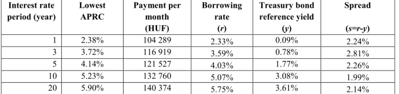
Suppose a Hungarian individual planning to take up a 20-year Hungarian forint (HUF) denominated mortgage loan of 20 M HUF to finance the purchase of a new home of 30 M HUF (≈100 000 EUR). Searching the internet, he/she gets several offers from different banks and for different interest rate periods. The structures with the lowest annual percentage rate of charge (APRC) are presented in Table 1.
Table 1: Best mortgage offers in Hungary (20 years, 20 M HUF, 16.07.2017)
Interest rate period (year)
Lowest APRC
Payment per month (HUF)
Borrowing rate
(r)
Treasury bond reference yield
(y)
Spread
(s=r-y)
1 2.38% 104 289 2.33% 0.09% 2.24%
3 3.72% 116 919 3.59% 0.78% 2.81%
5 4.14% 121 527 4.03% 1.77% 2.26%
10 5.23% 132 760 5.07% 3.08% 1.99%
20 5.90% 140 374 5.75% 3.61% 2.14%
Source: www.bankracio.hu, www.akk.hu
Now, he/she has to decide which interest rate period to choose. In the case of adjustable-rate (or variable-rate or floating rate) mortgages (ARM), the borrowing rate r is not fixed for the whole maturity but only for a shorter period by the end of which it is reset in accordance with a predefined reference yield (benchmark or index) y. The spread s, i.e. the difference between r and y can be constant
𝑟𝑡= 𝑦𝑡+ 𝑠 (1)
or proportional to the reference yield
𝑟𝑡 = 𝑦𝑡∙ 𝑘 (2)
4 where s>0 and k>1.2 Usually, the reference yield is the Hungarian interbank lending rate (BUBOR), or an interest swap rate, or a Treasury-bill or bond rate etc. Disregarding the slight differences between these quantities, we supposed in Table 1 that the reference yield is the sovereign HUF bond rate (its yield to maturity) corresponding to the given interest rate period.
Fixed rate mortgages (FRM) are risky because nominal payments are fixed, but their present value changes depending on the market conditions (present value risk). ARM loans are risky, too, as nominal payments change in line with the reference yield (cash-flow risk). Households usually care much more about the cash-flow risk than the present value risk. The fundamental risk of an ARM loan is that a rise in the reference yield y increases the borrowing rate r according to (1) or (2), which increases the monthly payment, the payment-to-income (PTI) ratio (if the net income of the borrower does not keep pace), and consequently the probability of default. Shorter interest rate periods with a proportional spread are even more risky from this aspect.
On the other hand, as Table 1 shows, the APRC of the loans depends on the interest rate period. At the moment, in Hungary, longer interest rate periods go with significantly higher APRC, which is mainly due to the shape of the reference yield curve. The difference between long and short term yields reflected also in APRCs is around 3.5%.
Financial awareness campaigns keep emphasizing that different loan structrures should be compared against the APRC measure as it contains all relevant costs of borrowing (Parker and Shay, 1974; Soto, 2013). Banks are required to disclose APRC during the whole credit agreement process. Web pages providing information for borrowers also stress the importance of this measure. When comparing loan conditions, APRC is always in the focus highlighted in large capital letters. Hence, borrowers are “trained” to minimize APRC even if it goes with higher risks, see the new home loan trends is Hungary in Table 2.
Table 2: New home loans in Hungary, 2016 and 2017Q1-Q2
Number Value
(thousand) (billion HUF)
Maturity ≤ 5 years 26 63
Maturity > 5 years 100 703
- adjustable-rate loans 69 556
- interest period is 1 year or shorter 35 304 Source: National Bank of Hungary
In the case of home loans with longer maturity than 5 years, a vast majority (69%) of the Hungarian borrowers chose adjustable-rate structures in the last 18 months. More than the
2 In Hungary, the Act on Fair Banking allows proportional spreads for interest rate periods of 3, 4, 5, and 10 years where k=1.25 according to the H1K standard.
5 half of these loans has 1-year or shorter interest rate period. If we consider the value of these contracts, these ratios are even higher.
We can see in Appendix II that typical PTI and LTV ratios are around 25% and 75%, respectively. As the current regulation stipulates that PTI and LTV cannot exceed 50% and 80%, respectively, LTV constraints seem more binding than PTI ones.
Appendices I and II also show that larger loans tend to have longer maturity, shorter interest rate period, higher PTI, and higher LTV. This is consistent with the empirical findings of van Ooijen and van Rooij (2016) that richer people with higher financial literacy can afford higher loans and higher risk because they can easily cope with financial problems should monthly payments arise. However, in the Hungarian case, it is hard to believe that 69% of homeowners choosing ARM loans (most of them with extremely short interest period) are aware of the corresponding risks and can really afford to undertake them. The predominance of ARM loans can be rather the sign of excessive risk taking and a myopic attitude in line with the empirical findings of Gathergood and Weber (2017) who showed that borrowers with poor financial literacy and “present bias” tend to choose riskier mortgage structures.
The seemingly contradictory results of van Ooijen and van Rooij (2016) versus Gathergood and Weber (2017) can be reconciled if we define three levels of financial literacy. The first level is when borrowers know nothing about finance; the second level is when borrowers are aware of APRC and think that this measure is to be minimized in any circumstances; and finally, the third level is when borrowers evaluate costs and risks carefully and optimize their strategy at least in these two dimensions. A change in financial literacy from the first to the second level may even increase excessive risk taking as APRC minimization usually goes with risk maximization; while a step from the second to the third level decreases it probably.
Therefore, contrary to the assumption behind multivariate regression models applied in the above studies, risk taking behavior might be a nonlinear and even non-monotone ∩-shape function of financial literacy. Different authors may report on different sides of this function.
The driving factors behind risk taking in the mortgage market were extensively investigated in the literature. Dhillon et al. (1987) found that when deciding on the loan structure, borrowers focus mainly on the pricing of the loans, i.e. they are simply minimizing the APRC. Co-borrowers, married couples, and short expected housing tenures were even more for adjustable-rate mortgages; while other characteristics like age, education, first-time home- buying, and self-employment were insignificant. Posey and Yavas (2001) proved in their theoretical model that under asymmetric information, rational high-risk (low-risk) borrowers choose ARM (FRM), thus, their choice can serve as a screening mechanism for the lender.
Kornai et al. (2003) explained excessive risk taking by the “soft budget constraint syndrome”, i.e. market players expecting external financial assistance with high probability are prone to undertake too much risk.
Based on the literature, we can conclude that the predominance of ARM loans with extremely short interest period can be the result of various reasons, but one of the major problems is that
6 a mass of half-educated borrowers concentrate solely on APRC minimizing while they believe to act rationally. In any case, rational or not, excessive risk taking is suboptimal at a social level, hence, regulators should intervene on behalf of the wider society.
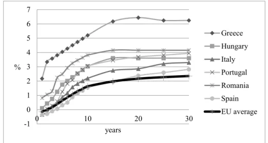
Clearly, the predominance of risky ARM loans is not just a Hungarian specialty; similar tendencies may arise in other countries, as well, especially, where the yield curve is sharply increasing. Figure 1 presents sovereign yield curves in the home currency across the EU.
Figure 1: Steepest and average reference yield curves in the European sovereign bond market (in home currency)
Source: Bloomberg, 18.07.2017.
Remark: Missing data were estimated by linear inter- and extrapolation.
The highest difference between long and short term rates in the Treasury market in the EU can be found in Portugal (4.2%), Greece (4.1%), Italy (3.6%), Hungary (3.5%), Romania (3.3%), and Spain (3.2%), whereas the EU average is 2.49%. Therefore, regulators should monitor mortgage markets’ tendencies in these countries very carefully.
ARM borrowers play the same yield curve game as Orange County (California, US) did in the 90’s. They are speculating on the future shape of the yield curve expecting lower future interest rates than the actual implicit forward ones. The only difference is that most of the ARM borrowers are investing in real estate and not in long term Treasury bonds. After some years of prosperity, Orange County became bankrupt, and its case serves as an excellent textbook example of irresponsible investment strategies (Hull, 2012).
3. Scenario analysis
To demonstrate why short interest rate periods are so dangerous at a systemic level, we performed a scenario analysis for the Hungarian case. Scenarios are defined in terms of the reference yield y prevailing at the end of the first interest rate period. The output of the
-1 0 1 2 3 4 5 6 7
0 10 20 30
%
years
Greece Hungary Italy Portugal Romania Spain EU average
7 analysis is the increase in the monthly payment which has a direct effect on the family’s living conditions, the ability-to-pay, and the default probability.
We assume that the spread is constant as in (1) and the Fisher-formula holds:
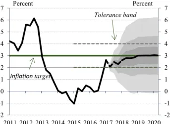
(1 + 𝑖𝑛𝑓𝑙𝑎𝑡𝑖𝑜𝑛 𝑟𝑎𝑡𝑒) ∙ (1 + 𝑟𝑒𝑎𝑙 𝑖𝑛𝑡𝑒𝑟𝑒𝑠𝑡) − 1 = 𝑟𝑒𝑓𝑒𝑟𝑒𝑛𝑐𝑒 𝑦𝑖𝑒𝑙𝑑 (3) Regarding the inflation rate, we rely on the latest inflation forecast of the Hungarian National Bank, see Figure 2.
Figure 2: Inflation rate forecast of the Hungarian National Bank, June 2017
Source: National Bank of Hungary (2017, Figure C1-1)
Figure 2, shows that the inflation rate is expected to increase to 2.8% in 2018, to 3% in 2019, and is supposed to remain stable afterwards. Different colors represent probability zones of 30%, 60%, and 90%. Note the high uncertainty even for shorter horizons.
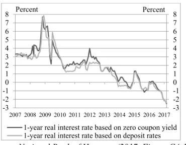
Regarding the real interest rate, official forecasts were not available; hence, we examined past time series, see Figure 3.
-2 -1 0 1 2 3 4 5 6 7
-2 -1 0 1 2 3 4 5 6 7
2011 2012 2013 2014 2015 2016 2017 2018 2019 2020
Percent Percent
Inflation target
Tolerance band
8 Figure 3: Real interest rate in Hungary, 2007-2017
Source: National Bank of Hungary (2017, Figure C4-10)
Similarly to worldwide tendencies, presently, the forward looking real interest rate is negative (-2.5%) and is at its historical minimum. In the last decade, the average real interest rate was around 2%, but the volatility was high (which is true for the whole last century). History also suggests that negative real interest rates are rare and only temporary.
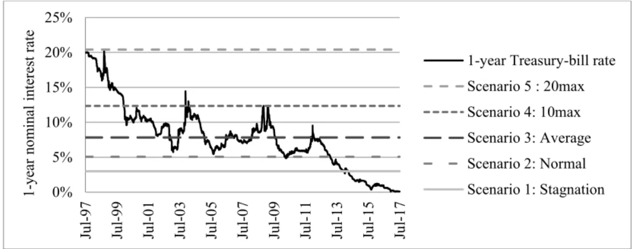
Based on these observations, we formulate five scenarios in Table 3.
Table 3: Scenarios of the future level of reference yields
Name Reference yield Remark
Scenario 1 Stagnation 3.00% 3% inflation and 0% real interest rate Scenario 2 Normal 5.06% 3% inflation and 2% real interest rate Scenario 3 20average 7.83% 20-year average of 1-year T-bill rate
Scenario 4 10max 12.35% 10-year maximum of 1-year T-bill rate
Scenario 5 20max 20.42% 20-year maximum of 1-year T-bill rate
The first scenario relies on the inflation forecast of the National Bank (3%) and supposes an interest rate (0%) which is consistent with an economic stagnation. The second scenario assumes the same inflation rate (3%), but the real interest rate is expected to return to its long term average (2%), which is consistent with normal economic conditions and is close to the 10-year average of the 1-year nominal interest rates. The third scenario simply takes the 20- year average (7.83%). Finally, the fourth and fifth scenarios reflect the 10-year and 20-year maximums (12.35% and 20.42%), respectively, see Figure 4.
-3 -2-1 0 1 2 3 4 5 67 8
-3 -2-1012345678
2007 2008 2009 2010 2011 2012 2013 2014 2015 2016 2017 Percent Percent
1-year real interest rate based on zero coupon yield 1-year real interest rate based on deposit rates
9 Figure 4: The 1-year nominal interest rate and the corresponding scenarios, 1997-2017
Source: www.portfolio.hu
Starting from the loan offers in Table 1, the results of the scenario analysis are presented in Table 4.
Table 4: Results of the scenario analysis, percentage change in payments, constant spread
Increase in payments at the end of the first interest rate period Interest rate period
(in years)
Initial borrowing rate
Scenario 1 y=3%
Scenario 2 y=5.06%
Scenario 3 y=7.83%
Scenario 4 10 y=12.35%
Scenario 5 y=20.42%
1 2.33% 28% 49% 81% 139% 253%
3 3.59% 18% 36% 62% 109% 201%
5 4.03% 9% 24% 46% 85% 164%
10 5.07% 0% 9% 23% 48% 97%
20 5.75% 0% 0% 0% 0% 0%
Table 4 shows the percentage change in the monthly payments at the end of the first interest rate period under different structures and scenarios. The shorter the interest rate period is and the higher the reference yield rises, the more the monthly payment of borrowers increases for the next interest rate period. For example, if the interest rate period is only 1 year, then modest scenarios like 1, 2, and 3 increase the payment by 28%, 49%, and 81%, respectively, which puts the ability-to-pay of the borrowers in serious danger. If the net income does not change, then PTI increases by the same ratio, e.g. if it was initially 50%, then the new PTI will be 64%, 75%, or 91%, which makes the loan almost impossible to repay. Scenarios 4 and 5 are more likely to get realized in the longer run, but their effect can be detrimental even though the remaining maturity of the loan will be relatively shorter by then.
According to the empirical literature, the default rate of ARM loans depends mainly on the payment-to-income (PTI) and loan-to-value (LTV) ratios which are related to the ability-to- pay and the willingness-to-pay, respectively (Banai et al. 2015; Connor and Flavin 2015).
Therefore, when evaluating the systemic risk in ARM lending, we have to consider also the net income of the households and the value of the real estate serving as collateral besides the
0%
5%
10%
15%
20%
25%
Jul-97 Jul-99 Jul-01 Jul-03 Jul-05 Jul-07 Jul-09 Jul-11 Jul-13 Jul-15 Jul-17
1-year nominal interest rate
1-year Treasury-bill rate Scenario 5 : 20max Scenario 4: 10max Scenario 3: Average Scenario 2: Normal Scenario 1: Stagnation
10 mortgage payment. In normal conditions, the increasing inflation rate increases not only the mortgage payments but also the incomes and house prices, which provide a natural hedge against inflation risk. However, the extent and the timing of these effects may be very different and it is not guaranteed that this relationship holds for short period and for all borrowers, at all. A macro level shock of increasing oil prices, stagnating economy, weakening home currency, sticky wages etc. may create an extremely adverse situation for ARM borrowers.
Even if the probabilities of scenarios in Table 4 are believed to be low, borrowers are certainly not able to evaluate these risks properly and a mass of households are taking too large speculative positions jeopardizing their living existence.
4. Adjustable-rate versus foreign currency mortgages
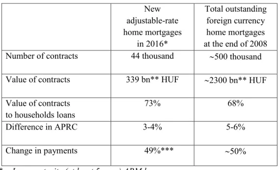
In this section, we demonstrate that adjustable-rate, home currency denominated mortgages are comparable to fixed rate, foreign currency denominated loans in terms of their riskiness and social impact. We can see in Table 5 how the new ARM loans of just the single year 2016 relate to the total foreign currency loan portfolio at the burst of the crisis which was accumulated for 4-5 years.
Table 5: Comparison of home mortgage booms in Hungary New
adjustable-rate home mortgages
in 2016*
Total outstanding foreign currency home mortgages at the end of 2008
Number of contracts 44 thousand 500 thousand
Value of contracts 339 bn** HUF 2300 bn** HUF Value of contracts
to households loans
73% 68%
Difference in APRC 3-4% 5-6%
Change in payments 49%*** 50%
* Long maturity (at least 5-year) ARM loans
** Billion is 10^9 according to the US terminology
***Estimation for a loan of 20-year maturity and 1-year interest rate period under Scenario 2 corresponding to normal economic conditions
(inflation=3%, real interest rate=2%) Source: National Bank of Hungary
11 Though it is hard to compare the recently started ARM housing boom to the fully developed foreign currency debt portfolio at the end of 2008, the new tendencies can easily lead to a similar crisis.
Note that adjustable-rate loans are as popular nowadays as foreign currency loans were in 2004-2008 not least because ARM loans help to reduce APRC by 3-4% points, which is considerable at the actual, fairly low level of borrowing rates. The increase of the payments under Scenario 2 (20-year maturity ARM with 1-year-long interest rate period) is roughly the same (49%) as the average increase was in the payments of CHF denominated loans (around 50%) which led to a deep and extensive social and economic crisis in 2008-2015 and ended up with massive bailout programs and a compulsory HUF conversion (Bethlendi, 2011;
Király and Simonovits, 2017).
To quantify which of the two structures has a higher cash-flow risk (i.e. the risk of increasing payments), suppose an adjustable-rate loan to be repaid in equal installments C, where payments are due at the end of each period ∆𝑡, and the borrowing rate r is reset right after the payments. We are at the moment to determine the borrowing rate r for the next period and we examine how the change in the reference yield y modifies the next payment C.
Consider first a loan of a similar structure, but with borrowing rate r fixed at the actual level for the whole maturity. The present value (or the price) of the loan P is
𝑃 = 𝐶 ∙ 𝐴 (4)
where 𝐴 = 𝐴(𝑟, 𝑇) is the annuity factor. The price sensitivity i.e. the percentage change in price for a unit change in yield is the so-called modified duration 𝐷∗ (Bodie, Kane, and Marcus 2014):
𝑑𝑃/𝑃
𝑑𝑟 = −𝐷∗ (5)
Clearly, 𝐷∗ > 0 as an increase in the interest rate leads to a decrease in the present value. It follows from (4) and (5) that
𝑑𝑃
𝑑𝑟 = −𝐷∗∙ 𝑃 = 𝐶 ∙𝑑𝐴 𝑑𝑟
(6)
and 𝑑𝐴𝑑𝑟 < 0. We can express 𝑑𝐴𝑑𝑟 from (6) as 𝑑𝐴
𝑑𝑟 =−𝐷∗∙ 𝑃 𝐶
(7)
12 Since 𝑑𝐴𝑑𝑟 depends only on r and T, therefore, (7) remains valid for adjustable-rate loans, as well (where 𝐷∗ is still the modified duration of the fixed loan). For the adjustable-rate loan, (4) holds, as well, but now the present value of the loan P is fixed and the next payment C changes in accordance with the borrowing rate r:
𝐶 = 𝑃 𝐴(𝑟, 𝑇)
(8)
Using (8) and (7), we calculate the semi-elasticity of C to r, i.e. the percentage change in payment for a unit change in the borrowing rate:
𝑑𝐶/𝐶 𝑑𝑟 = −
𝑑𝐴𝑑𝑟 𝐴 =
𝐷∗∙ 𝑃 𝐶
𝐴 = 𝐷∗
(9)
Hence, by (9), the rate sensitivity of the payment is the same as the modified duration of a similar but fixed loan calculated at the present borrowing rate. Note that Király and Simonovits (2017) derive the same formula but in a more complicated form and they do not link it to the modified duration. Our approach has also the advantage that the modified duration is an intuitive, widely-used, and easily-computable measure.
Now, we show the effect of the reference yield y on the payment C. This effect depends on the spread algorithm, i.e. on the relationship between r and y. We consider the general formula
𝑟 = 𝑦 ∙ 𝑘 + 𝑠 (10)
where 𝑘 ≥ 1 and 𝑠 ≥ 0. This contains the special cases of (1) and (2), i.e. the constant and the proportional spreads, for 𝑘 = 1, 𝑠 > 0, and 𝑘 > 1, 𝑠 = 0, respectively.
By (10), we have 𝑑𝑟 = 𝑑𝑦 ∙ 𝑘. Hence, by (9), the semi-elasticity of C to y is 𝑑𝐶/𝐶
𝑑𝑦 = 𝑑𝐶/𝐶
𝑑𝑟/𝑘 = 𝐷∗∙ 𝑘 (11)
It follows from (11) that proportional spreads are much more dangerous than constant spreads. Table 4 above showed the scenario analysis for loans with a constant spread. In the case of proportional spreads, values in Table 4 should be multiplied with k>1.
Of course, the first derivative of a function characterizes only the effect of a small change. It can be shown that C is a strictly convex function of y for the entire relevant domain, hence
∆𝐶/𝐶
∆𝑦 > 𝑑𝐶/𝐶 𝑑𝑦
(12)
13 Note that convexity is against the borrower; thus, increases in payments (for example in Table 4) are larger than formula (11) suggests.
To sum up, the cash-flow risk of an adjustable-rate loan can be approximated by the modified duration of the corresponding fixed loan. It follows from (11) that a change of 100 basis points in the reference yield y causes a change of 𝐷∗∙ 𝑘 % in the payment. For example, in the case of the first loan of Table 1 where the initial maturity is 20 years, the interest rate period is 1 year, and the initial borrowing rate is r=y+s=0.09%+2.24%=2.33%, 𝐷∗=9.09 at the end of the first year. This means that a 100-basis-point upward shift in the reference yield y (from 0.09% to 1.09%) will increase the payment C at least by 9.09% for a constant spread and by 9.09%∙1.25=11.36% for a proportional spread with k=1.25 set by the Act on Fair Banking in Hungary.
If this loan were denominated in Swiss franc (CHF) and the borrowing rate were fixed, then the main risk factor would be the exchange rate X, i.e. the CHF/HUF rate. The payment C would be a linear function of the exchange rate X and 1% change in X would cause exactly 1% change in C. Hence, a percentage change in X has the same effect on the payment as 𝑑𝑦 ∙ 𝐷∗∙ 𝑘 unit change in the reference yield:
𝑑𝐶/𝐶 = 𝑑𝑋/𝑋 = 𝑑𝑦 ∙ 𝐷∗∙ 𝑘 (13)
Therefore, in the case of the first loan in Table 1, a 100-basis-point change in the reference yield (1-year T-bill yield) is equivalent to 9.09% change in the CHF/HUF rate (or to 11.36%
if we have a proportional spread). Let us examine which event tends to happen more frequently.
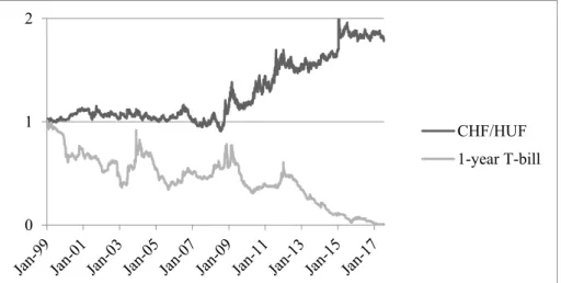
Figure 5: Basis index of CHF/HUF rate and 1-year Treasury-bill rate, 01.01.1999-07.17.2017
Source: www.portfolio.hu
0 1 2
CHF/HUF 1-year T-bill
14 In the last 18.5 years3, the CHF/HUF rate increased by approximately 100% (doubled) while the 1-year T-bill rate decreased by approximately 100% (dropped to near zero).
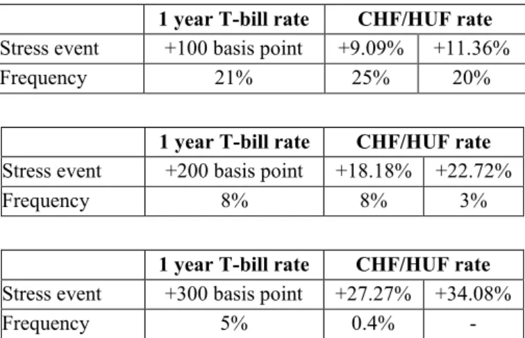
Supposing that both CHF returns and T-bill rate changes come from identical distributions, we can compare which stress event was more frequent in this past period: a more than 100- basis-point increase in the 1-year reference yield or a more than 9.09% (or 11.36%) increase in the Swiss franc rate. In Table 6 we present the frequencies also for the double and triple size stress events.
Table 6: Frequency of equivalent stress events, 01.01.1999-07.17.2017
1 year T-bill rate CHF/HUF rate Stress event +100 basis point +9.09% +11.36%
Frequency 21% 25% 20%
1 year T-bill rate CHF/HUF rate Stress event +200 basis point +18.18% +22.72%
Frequency 8% 8% 3%
1 year T-bill rate CHF/HUF rate Stress event +300 basis point +27.27% +34.08%
Frequency 5% 0.4% -
According to Table 6, the frequency of equivalent stress events tended to be the same or even higher in the T-bill than in the CHF market. This is especially true if we take more serious stress events. For example, the maximum of yearly change in the T-bill rates was around 700 basis points (in 2012-2013) which is equivalent to 7%*9.09 = 63.63% change in the CHF rate but the maximum of the latter was only 34% (in 2008-2009). Thus, in the last 18.5 years, it would have been somewhat safer to borrow in CHF but at fixed interest rate than to borrow in HUF but at adjustable rate with 1-year interest period, especially, if the ARM spread is proportional and we consider the effect of convexity, as well.
At the moment, the outlook for ARM loans is worse than in the past, because interest rates are near to zero; hence, there is no more potential in decreasing. The best thing that can happen to ARM borrowers is that interest rates remain approximately the same. A significant increase in the reference yields may not seem very likely in the short run, but unexpected external shocks may boost the inflation and nominal rates in the longer run. Real interest rates being at their historical minimum, too, can be expected to increase, as well. If interest rates will be as volatile in the future as in the past, then ARM borrowers should really prepare for the worst scenarios.
In the above analysis, we concentrated only on the risk of increasing PTIs, i.e. the cash-flow risk of borrowers which turned to be approximately the same for CHF denominated fixed
3 CHF/HUF data were not available before 1999.
15 loans and home currency ARM loans. However, if we consider the risk of increasing LTVs, as well, foreign currency borrowing is definitely riskier as the depreciation of the home currency increases not only the repayments but also the present values of the debts. This is not true for ARM loans because an increase in the nominal rates leaves the debts unchanged, moreover, rising inflation generally increases home prices; thus, LTVs tend to decrease in a stress situation.
However, when evaluating the overall systemic effects of ARM loans, we have to differentiate between families living in their homes and profit-seeking, highly-leveraged investors. In the latter case, ARM loans provide a natural hedge against inflation indeed, since rising repayments are compensated by rising investment value and the cash-flow risk can be easily managed on the capital markets. However, in the case of simple households, increasing inflation is not immediately offset by increasing nominal incomes; therefore, their living existence is seriously menaced and decreasing LTVs help only the lender institutions. Thus, regarding the social effects, ARM loans can be as much detrimental as currency denominated fixed loans.
5. Our proposition: risk-adjusted APRC
In the aftermath of the global crisis of 2007-2008, various new financial regulations were invented and implemented worldwide to control systemic risk, to make economic institutions more resilient and to protect consumers; thus, banks’ lending activity is much more regulated and transparent than before.
In spite of these measures, however, excessive risk taking behavior may reappear in different guises, for example in the form of adjustable rate mortgages as in Hungary. This can be explained by many factors, but to a large extent it is due to the misleading calculation of the annual percentage rate of charge (APRC).
APRC calculation is regulated according to Directive (2014/17/EU) throughout the European Union. The aim of the regulation was to make different types of credit comparable. It is calculated as an internal rate of return where future cash-flows 𝐶𝑡 are the payments of the borrower and the present value PV is the face value of the loan
𝑃𝑉 = ∑ 𝐶𝑡 (1 + 𝐴𝑃𝑅𝐶)𝑡
𝑇
𝑡=1
(14)
Although there are several complications regarding cost elements (e.g. interest rates, administration fees, mortgage registration) and time conventions, especially, in credit agreements where there are different draw-down and repayment options, grace periods etc., these features are exhaustively discussed in the directive.
16 Soto (2013, page 56) formulates the main advantage of APRC as “… it puts the credit, its costs and time together, thus recognizing that these three elements are relevant in determining a comparable and uniform measure of the cost of the credit. In this way, the APR presents significant advantages over other measures of cost.”
However, an important assumption what makes APRC calculation totally misleading is that initial conditions are assumed to remain fixed: “In the case of credit agreements containing clauses allowing variations in the borrowing rate and, where applicable, in the charges contained in the APRC but unquantifiable at the time of calculation, the APRC shall be calculated on the assumption that the borrowing rate and other charges will remain fixed in relation to the level set at the conclusion of the contract.” (Directive, 2014/17/EU, 16(4)) For example, in the case of an adjustable-rate mortgage, future cash-flows 𝐶𝑡 in (14) are determined according to the present borrowing rate r, while in the case of a foreign currency denominated loan, it is assumed that the FX rate X will be the same as today throughout the whole lifespan of the loan:
𝑃𝑉 = ∑ 𝐶𝑡
(1 + 𝐴𝑃𝑅𝐶)𝑡 = ∑𝑁𝑡−1∙ 𝑟0∙ 𝑋0+ 𝑅𝑡∙ 𝑋0+ 𝑀𝑡 (1 + 𝐴𝑃𝑅𝐶)𝑡
𝑇
𝑡=1 𝑇
𝑡=1
(15)
where 𝑟0 is the borrowing rate at t=0, 𝑋0 is the FX rate at t=0 (𝑋0=1 if the loan is denominated in home currency), 𝑁𝑡 is the nominal value of the loan, 𝑅𝑡 is the repayment of the principal, and 𝑀𝑡 is the administrative cost due at the end of period t.
In this way, APRC reflects the charges of the loan but tells nothing about the risk that r and X change over time. However, if APRC is a standardized tool developed explicitly to help borrowers to compare different loan contracts, it should be risk-adjusted. Borrowing is the reverse of investing. When evaluating different investment opportunities, it is obvious that we use risk-adjusted performance measures and not only the expected return in itself. Similarly to this, borrowing opportunities should also be evaluated according to their riskiness, as well, and not only to their charges. A new measure is needed which comprehends both concepts and defines a trade-off between them, too.
Directive (2014/17/EU) prescribes to inform borrowers about risks, as well, but it is a separate and much less pronounced calculation: "Where the credit agreement allows for variations in the borrowing rate, Member States shall ensure that the consumer is informed of the possible impacts of variations on the amounts payable and on the APRC at least by means of the European Standardised Information Sheet (ESIS). This shall be done by providing the consumer with an additional (stressed) APRC which illustrates the possible risks linked to a significant increase in the borrowing rate." 16(6) of (Directive, 2014/17/EU)
The risk is expressed as a result of a predefined stress test: “Where there is a cap on the borrowing rate, the example shall assume that the borrowing rate rises at the earliest possible opportunity to the highest level foreseen in the credit agreement. Where there is no
17 cap, the example shall illustrate the APRC at the highest borrowing rate in at least the last 20 years.” (Directive, 2014/17/EU, Annex II. Part B, Section 4(2)) However, this measure is quite difficult to understand, for example, it does not inform directly about the increment in the monthly payment and gives no guideline how to judge the relevance of the stress scenario, i.e. the borrowing rate reaching its 20-year maximum in the near future. Even if borrowers understood the concept of the stressed APRC, it is not obvious how to rank against two conflicting measures at the same time, and they may have troubles in defining the trade-off between plain APRC and stressed APRC properly. Another problem with stressed APRC is that it is not accentuated in the initial advertising phase at all. As internet websites specialized in the comparison of mortgage loans do not indicate any risk measures, different loans can be ranked simply by the charges (APRC, monthly payment, administration fees). Stressed APRC appears only in small letters on the information sheet clients get from the bank in the pre- contractual phase, when they have almost decided which loan to take.
Our proposition is to introduce a single measure, the risk-adjusted APRC to rank credit offers.
The idea is that uncertain future variables (borrowing rates r and FX rates X) should be replaced in formula (15) by the suitable forward rates:
𝑃𝑉 = ∑ 𝐶𝑡
(1 + 𝐴𝑃𝑅𝐶)𝑡 = ∑𝑁𝑡−1∙ 𝑓𝑡−1,𝑡∙ 𝐹𝑡+ 𝑅𝑡∙ 𝐹𝑡+ 𝑀𝑡 (1 + 𝐴𝑃𝑅𝐶)𝑡
𝑇
𝑡=1 𝑇
𝑡=1
(16)
where 𝑓𝑡−1,𝑡 is the forward interest rate for the period between t-1 and t, and 𝐹𝑡 is the forward price of the foreign currency for the end of period t valid at the initiation of the loan contract t=0. Though forward rates are not necessarily equal to the expected values of future rates, they can still be introduced into formula (16) since they are the certainty equivalents (CEQ) of the future rates, i.e. the present values of the two are equivalent. The same CEQ method is applied during the valuation of derivative contracts (e.g. swaps) many times, as well, see Hull (2012).
The corresponding article of the directive (Directive, 2014/17/EU, 16(4)) should be modified accordingly: “In the case of credit agreements containing clauses allowing variations in the borrowing rate and, where applicable, in the charges contained in the APRC but unquantifiable at the time of calculation, the risk-adjusted APRC shall be calculated on the assumption that the borrowing rate and other charges will remain fixed in relation to the level set at the conclusion of the contract change according to their reference forward rates.”
The reference forward rates can be calculated from the reference yield curves or can be determined and published directly by the regulator on a daily basis.
The fundamental disadvantage of the plain APRC is that it contains not only the charges of the loan, but also the risk premium the borrower gets in exchange of the undertaken risks.
These risks, however, can be switched off with the help of forward contracts, as we suggest.
In this way, eliminating the risk premium component and reflecting only the pure charges,
18 such as spreads and administration costs, the risk-adjusted APRC makes loan offers really comparable. Note that this is true independently of the actual form of the yield curve.
A similar concept lies behind the well-known risk-adjusted performance measure Jensen- alpha 𝛼𝑖, as well, which indicates the excess return of the ith portfolio relative to the Capital Asset Pricing Model (CAPM):
𝛼𝑖 = 𝑟𝑖− (𝑟𝑓+ 𝛽𝑖 ∙ 𝑀𝑅𝑃) (17) where 𝑟𝑖 is the average return of the portfolio, 𝑟𝑓 is the risk-free rate, 𝛽𝑖 measures the portfolio’s market risk, and MRP is the average market risk premium (Bodie, Kane, and Markus, 2014). It can be easily shown that Jensen-alpha is the residual return of the portfolio if we properly hedge the market risk, i.e. switch off the risk-premium, for example by shorting index futures.
Consequently, risk-adjusted APRC can be interpreted similarly to the present plain APRC with the difference that it really contains all charges including even the costs of risk hedging.
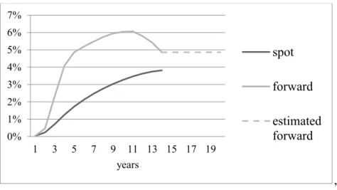
It is a natural idea in finance to convert risks into costs (and vice versa) and the calculation is simple as far as the hedging instruments are traded and their prices can be determined, i.e. the markets are complete. Indeed, if clients hedged the risk of variable reference yields and FX rates in the forward (or futures) markets, and the costs of hedging were also considered according to (16), then the virtual advantage of adjustable-rate and foreign currency loans would immediately disappear. To illustrate this, let us take the spot and the one-year forward rate curves in Hungary, see Figure 6.
Figure 6: Spot and 1-year forward rates in the Hungarian Treasury bond market, 14.07.2017.
, Source: www.akk.hu
As the longest maturity of the spot yield curve is around 14.27 years, we simply suppose that the last forward rate (4.86) applies to the later periods. Assuming that payments are due only
0%
1%
2%
3%
4%
5%
6%
7%
1 3 5 7 9 11 13 15 17 19
years
spot forward estimated forward
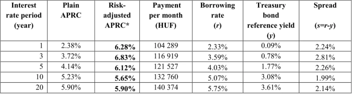
19 at the end of the year, we calculate the risk-adjusted APRC measures for the mortgage loans in Table 1 applying (16), see Table 7.
Table 7: Plain versus risk-adjusted APRC in Hungary (20 years, 20 M HUF, 2017.07.16)
Interest rate period
(year)
Plain APRC
Risk- adjusted
APRC*
Payment per month
(HUF)
Borrowing rate
(r)
Treasury bond reference yield
(y)
Spread (s=r-y)
1 2.38% 6.28% 104 289 2.33% 0.09% 2.24%
3 3.72% 6.83% 116 919 3.59% 0.78% 2.81%
5 4.14% 6.12% 121 527 4.03% 1.77% 2.26%
10 5.23% 5.65% 132 760 5.07% 3.08% 1.99%
20 5.90% 5.90% 140 374 5.75% 3.61% 2.14%
*Administration costs are not included as their cash-flows were not available.
Table 7 contains the same values as Table 1 with the exception of the new column showing risk-adjusted APRCs. These new measures are much more homogeneous than plain APRCs, their differences are due to the differences in spreads, but not to the shape of the reference yield curve anymore. In this example, we get that the 10 and 20-year fixed rate structures have the lowest risk-adjusted APRC, hence these two might be the most favorable for most of the borrowers. Banks seem to earn more and risk more on borrowers choosing shorter interest rate periods. Note that ranking should rely on the risk-adjusted APRC as all other popular measures, like payments per month, borrowing rates, reference yields, can be misleading, because these are temporary indicators prevailing only at the initiation of the contract.
6. Conclusions
In Hungary, right after the consolidation of the foreign currency mortgage crisis of 2008- 2015, a new home lending wave is starting off in 2016-2017 where 69% of the borrowers take HUF-denominated but adjustable-rate mortgages (ARM) and more than the half of them choose extremely short (1-year or less) interest rate periods. Based on the empirical literature of mortgage markets, we can assume that a large part of the borrowers is just minimizing APRC to save the difference of about 3.5% in the reference yields. Similar or even more accentuated yield curve patterns can be found in many other countries, as well, for example in Portugal, Greece, Italy, Romania, and Spain, which creates a strong motivation to borrow at very short interest rate periods.
Performing a scenario analysis, we show that a typical household cannot afford the risk of potentially increasing payments. If the interest rate period is 1 year and the spread is constant, then under realistic Scenarios 1, 2, and 3, payments increase by 28%, 49%, and 81%, respectively, which puts the ability-to-pay of the borrowers into serious danger. If the net income of the borrower does not change, then PTI increases by the same ratio, e.g. if it was initially 50% (according to the present regulation this is the maximum at the beginning of the
20 loan contract), then the new PTI will be 64%, 74.5%, and 90.5%, respectively, which makes the loan impossible to repay.
We also demonstrate that adjustable-rate mortgages are comparable to foreign currency denominated loans in terms of their cash-flow risk and social impact. With ARM loans, the gain in APRC is somewhat lower (3-4% versus 5-6%), but the weight of ARM loans within the total household loan portfolio is larger (73% versus 68%) and also the potential increase in payments is 49% which is approximately the same as experienced during the recent, foreign currency mortgage crisis.
To quantify the risk of ARM loans, we derive the semi-elasticities of the monthly payment to the borrowing rate and the reference yield. The first turns to be equal to the modified duration of a similar but fixed rate loan, while the second depends on the spread algorithm. If the spread is constant, then it is the modified duration again, however, in the case of a proportional spread, it is k times the modified duration, where k is the spread multiplier. The Hungarian Act on Fair Banking allows proportional spreads with k=1.25, which means that proportional-spread ARM loans comprehend also the hidden risk that payments will increase by 25% more than in the case of the constant-spread ARM loans. Thus, proportional spreads aggravate the perverse incentives of irresponsible risk-taking, and should not be tolerated by a prudent regulator.
Moreover, convexity is against the borrowers, hence, larger changes in the reference yields cause even larger changes in the payments than the modified duration would suggest. A useful rule of thumb for constant-spread ARM loans is that a 100-basis-point increase in the reference yield will increase the payments by a percentage of at least the half of the maturity of the loan (thus, for a 20-year loan, it is around 10%). Using this formula and examining past time series of T-bill and CHF/HUF rates, we conclude that in the last two decades in Hungary, households borrowing at a variable rate would have run slightly more cash-flow risk than those borrowing in Swiss franc.
The excessive risk taking of mortgage borrowers increases the systemic risk which has significant negative spill-over effects for the whole society. Regulators may control these phenomena in many ways. Our proposition is to introduce a new measure to rank credit products which reflects the pure charges of borrowing. We keep the basic logic of the present APRC formula; however, instead of assuming that uncertain variables (reference yields and FX rates) remain the same over time, we suggest to replace them with suitable forward rates, i.e. with their certainty equivalents (CEQ). In this way, we get the so called risk-adjusted APRC that can be interpreted similarly to the present plain APRC with the exception that now it really contains all costs of borrowing ˗ even the potential costs of risk hedging. It is a natural idea in finance to convert risks into costs. This conversion is simple as far as the hedging instruments are traded and their prices can be determined, i.e. markets are complete.
It follows from the proposed methodology that the risk-adjusted APRC reveals the hidden risk of proportional spreads, as well. We illustrate with the Hungarian case that the virtual advantage of adjustable-rate (or foreign currency) loans would immediately disappear if
21 clients hedged the risk of variable reference yields (or FX rates) in the forward markets and the costs of this hedging were included in the APRC calculation. Note that we do not suggest to hedge all interest and FX rate risks in effect, just to calculate the costs of a hypothetical hedging and to incorporate them into the new version of APRC.
Acknowledgement: The research was supported by the János Bolyai scholarship program of the Hungarian Academy of Sciences. We are very grateful to Tamás Makara for his inspiration and valuable comments. We also thank the National Bank of Hungary for the database of home loans in 2016-2017.
22 Appendix I.*
* ARM loans where interest rate periods are shorter than maturity are colored in grey.
(𝑎; 𝑏 ] means the interval 𝑎 < 𝑥 ≤ 𝑏.
I/A Number of new home contracts (thousands), 2016 and 2017Q1-Q2
Maturity in years
Interest rate period in years
(0;0.25] (0.25;1] (1;3] (3;5] (5;10] (10;20] (20;30] >30 Sum
(0;5] 1.4 2.5 5.3 16.6 - - - - 25.8
(5;10] 1.7 3.1 0.1 3.6 23.1 - - - 31.5
(10;15] 2.2 5.2 0.1 4.9 3.4 5.8 - - 21.6
(15;20] 2.2 6.4 0.1 5.5 2.1 1.6 - - 18.0
(20;25] 2.7 6.6 0.1 6.9 2.5 0.3 0.3 - 19.3
(25;30] 1.1 2.0 0.0 3.1 0.3 0.0 0.2 - 6.7
>30 0.7 0.8 - 0.8 0.1 - - 0.0 2.5
Sum 12.0 26.5 5.7 41.6 31.5 7.7 0.4 0.0 125.4
Source: National Bank of Hungary
I/B Value of new home loan contracts (billions, i.e. 10^9 of HUF), 2016 and 2017Q1-Q2
Maturity in years
Interest rate period in years
(0;0.25] (0.25;1] (1;3] (3;5] (5;10] (10;20] (20;30] >30 Sum (0;5] 4.0 7.7 15.1 36.5 - - - - 63.4 (5;10] 7.9 17.4 0.5 16.5 100.0 - - - 142.4 (10;15] 14.5 37.1 0.7 29.8 20.6 29.6 - - 132.2 (15;20] 20.5 59.4 1.2 40.9 16.1 13.6 - - 151.7 (20;25] 28.3 64.2 0.9 58.4 21.9 2.1 2.3 - 178.2 (25;30] 12.6 23.4 0.2 29.3 3.4 0.0 1.7 - 70.5
>30 8.9 9.7 - 8.1 1.2 - - 0.0 28.0 Sum 96.7 219.0 18.7 219.5 163.2 45.3 4.0 0.0 766.4
Source: National Bank of Hungary
I/C Average value of new home loan contracts (millions of HUF), 2016 and 2017Q1-Q2
Maturity in years
Interest rate period in years
(0;0.25] (0.25;1] (1;3] (3;5] (5;10] (10;20] (20;30] >30 Sum
(0;5] 2.9 3.1 2.9 2.2 2.5
(5;10] 4.8 5.7 5.6 4.5 4.3 4.5
(10;15] 6.6 7.2 6.5 6.0 6.0 5.1 6.1
(15;20] 9.2 9.3 8.8 7.4 7.7 8.4 8.4
(20;25] 10.5 9.8 10.0 8.4 8.8 7.6 8.6 9.2
(25;30] 11.2 11.6 11.4 9.4 11.2 12.3 10.7 10.5
>30 12.8 11.5 10.0 11.5 5.9 11.3
Sum 8.1 8.3 3.3 5.3 5.2 5.9 9.4 5.9 6.1
Source: National Bank of Hungary
23 Appendix II.
II/A Frequency of PTI (payment-to-income) of new home loans, 2016 and 2017Q1-Q2
Source: National Bank of Hungary
II/B Frequency of LTV (loan-to-value) of new home loans, 2016 and 2017Q1-Q2
Source: National Bank of Hungary
0%
2%
4%
6%
8%
10%
12%
14%
16%
18%
5 10 15 20 25 30 35 40 45 50 55 60 65
frequency
PTI (%)
number value
0%
2%
4%
6%
8%
10%
12%
5 20 35 50 65 80 95 110 125 140 155
frequency
LTV(%)
number value
24 References
Bethlendi, A. (2011). Policy measures and failures on foreign currency household lending in Central and Eastern Europe. Acta Oeconomica. 61(2): 193-223.
Bodie, Z.; Kane, A.; Marcus, A. J. (2014). Investments. McGraw-Hill Education
Connor, G.; Flavin, T. (2015). Strategic, unaffordability and dual-trigger default in the Irish mortgage market. Journal of Housing Economics. 28: 59-75.
Dhillon, U. S. Shilling, J. D., Sirmans, C. F., (1987). Choosing between fixed and adjustable rate mortgages. Journal of Money, Credit and Banking. 19(2): 260-267.
Directive (2008/48/EU). Directive 2008/48/EC of the European Parliament and of the Council of 23 April 2008 on credit agreements for consumers and repealing Council Directive
87/102/EEC.
http://eur-lex.europa.eu/LexUriServ/LexUriServ.do?uri=OJ:L:2008:133:0066:0092:EN:PDF Accessed: 08.10.2017
Directive (2014/17/EU). Directive 2014/17/EU of the European Parliament and of the Council on credit agreements for consumers relating to residential immovable property and amending Directives 2008/48/EC and 2013/36/EU and Regulation (EU) No 1093/2010
http://eur-lex.europa.eu/legal-content/EN/TXT/PDF/?uri=CELEX:32014L0017&from=en Accessed: 08.10.2017
Gathergood, J.; Weber, J. (2017). Financial literacy, present bias, and alternative mortgage products. Journal of Banking and Finance. 78: 58-53.
Hull, J. C. (2012). Options, futures, and other derivatives. 8th Edition, Pearson
Király, J.; Simonovits, A. (2017). Mortgages denominated in domestic and foreign currencies:
simple models. Journal of Emerging Markets Finance and Trade. 53(7): 1641-1653.
Kornai, J.; Maskin, E.; Roland, G. (2003). Understanding the soft budget constraint. Journal of Economic Literature. 41(4): 1095-1136.
National Bank of Hungary (2017): Inflation Report. June 2017
Parker, G. G. C.; Shay, R. P. (1974). Some factors affecting awareness of annual percentage rates in consumer installment credit transactions. The Journal of Finance. 29: 217-225.
Posey, L. L.; Yavas, A. (2001). Adjustable and fixed rate mortgages as a screening mechanism for default risk. Journal of Urban Economics. 49(1): 54-79.
25 Soto, M. G. (2013). Study on the calculation of the annual percentage rate of charge for consumer credit agreements, European Commission Directorate‐General Health and Consumer Protection
van Ooijen, R.; van Rooij, M. C. J. (2016). Mortgage risks, debt literacy, and financial advice.
Journal of Banking and Finance. 72: 201-217.