Evolutionary Substitution and Replacement in N-Species Lotka-Volterra Systems ∗
Ross Cressman
+,
Mikl´ os Koller
#, M. Barnab´ as Garay
#, J´ ozsef Garay
+++
Department of Mathematics Wilfrid Laurier University Waterloo, Ontario N2l 3C5 Canada
(e-mail: rcressman@wlu.ca)
#
Faculty of Information Technology and Bionics, P´ azm´ any P´ eter Catholic University,
Pr´ ater utca 50/A H-1083 Budapest, Hungary
(e-mail: koller.miklos@itk.ppke.hu, garay@itk.ppke.hu)
++
MTA Centre for Ecological Research, Evolutionary Systems Research Group, Klebelsberg Kuno utca 3, Tihany 8237, Hungary
and
MTA-ELTE Theoretical Biology and Evolutionary Ecology Research Group
and
Department of Plant Systematics, Ecology and Theoretical Biology,
E¨ otv¨ os Lor´ and University,
P´ azm´ any P´ eter s´ et´ any1/c, H-1117 Budapest, Hungary (e-mail: garayj@caesar.elte.hu)
April 3, 2019
Abstract
Abstract: The successful invasion of a multi-species resident sys- tem by mutants has received a great deal of attention in theoretical ecology but less is known about what happens after the successful in- vasion. Here, in the framework of Lotka-Volterra (LV) systems, we consider the general question where there is one resident phenotype in each species and the evolutionary outcome after invasion remains one phenotype in each species but these include all the mutant phenotype- s. In the first case, called evolutionary substitution, a mutant appears in only one species, the resident phenotype in this species dies out and the mutant coexists with the original phenotypes of the other species.
In the second case, called evolutionary replacement, a mutant appears in each species, all resident phenotypes die out and the evolutionary outcome is coexistence among all the mutant phenotypes. For general LV systems, we show that dominance of the resident phenotype by the mutant (i.e. the mutant is always more fit) in each species where the mutant appears leads to evolutionary substitution/replacement.
However, it is shown by example that, when dominance is weakened to only assuming the average fitness of the mutants is greater than the average for the resident phenotype, the residents may not die out.
We also show evolutionary substitution occurs in two-species com- petitive LV systems when the initial invasion of the resident system (respectively, of the new coexistence system) is successful (respective- ly, unsuccessful). Moreover, if sequential evolutionary substitution occurs for either order that the two mutant phenotypes appear (called historically independent replacement), then it is shown evolutionary replacement occurs using a generalization of the dominance argument.
Keywords: resident and mutant phenotypes, successful invasion, evolution- arily stable strategy, competitive Lotka-Volterra systems
∗Financial assistance from the Natural Sciences and Engineering Research Council (NSERC) of Canada (to R.C.) as well as from grants GINOP 2.3.2-15-2016-00057 (to J.G.) and NKFIH No 115926 (to M.B.G.) of Hungary is gratefully acknowledged. This project has also received funding from the European Union’s Horizon 2020 research and innovation programme under the Marie Sk lodowska-Curie grant agreement No 690817.
1 Introduction
1
In this paper, we consider a resident system with N species together with
2
a set of invaders. In order to motivate this setup, which is rooted in ecol-
3
ogy and evolution theory, we provide relevant examples here. In ecological
4
succession, after a disturbance (e.g. wildfire, lava flow or landslide), species
5
from an existing pool colonize the new habitat. During the succession pro-
6
cess, which starts with these pioneering plants and animals and stops when
7
a long-term stable community emerges, a number of species replace other
8
ones (Pielou 1966; Drake 1990). In ecological invasion theory, the hypothesis
9
of “invasional meltdown” proposes that an invasive species in a new envi-
10
ronment can facilitate the invasion of other non-native species (Simberloff
11
and Von Holle 1999). However, there are also examples when multispecies
12
invasion can reduce the negative impact of a single exotic plant species on
13
the native (i.e. resident) plant community (Lenda 2019).
14
Invasion by multiple species can happen through human activity or by
15
natural causes. For instance, the latter occurred during the formation of the
16
Isthmus of Panama when the migration between North and South America
17
led to the last and most conspicuous wave, the great American interchange,
18
around 3 million years ago (O’Dea et al. 2016; Stehli and Webb 2013). Fur-
19
thermore, sympatric speciation is the evolution of a new species from a sur-
20
viving ancestral species, while both live in the same habitat. An important
21
question is: What is the number of mutants in a large ecosystem? The num-
22
ber of co-existing mutants depends on the size of the ancestral species and
23
the time duration until extinction of non-successful mutants. In particular,
24
we cannot rule out the possibility that an already introduced non-successful
25
mutant can survive if a new mutant arises in another species, and together
26
can successfully invade the ancestral system.
27
From the biological perspective, there are two main differences between
28
evolutionary and ecological models. Firstly, in evolution, mutation is rare
29
in two senses; the mutant occurs with low density, and there is a long time
30
duration between two mutation events. In ecological models, more than one
31
invasive species can be introduced at (almost) the same time and in large
32
numbers either by accident or on purpose through human activities. Second-
33
ly, in evolution, the mutant phenotypes are not arbitrary, contrary to ecology
34
where the invasive species has arbitrary traits. Usually, during evolution, the
35
mutant and the wild phenotypes do not radically differ from each other. Of-
36
ten, the interaction parameters in the evolutionary model either come from
37
the same game and the phenotypes are different (see Cressman and Garay
38
2003a,b; Garay 2007) or interaction parameters between resident and mutant
39
phenotypes are not so different. This contrasts to models in invasion ecology
40
where the phenotypic similarity between exotic and native species cannot be
41
assumed. One well-known example of dissimilar phenotypes is from Australi-
42
a, when the invasive mammals substitute for the native marsupials. However,
43
Hutchinson (1965) has already emphasized that biotic evolution cannot be
44
separated from ecology, since ecological factors (like competition and feed-
45
ing) have a curtailing effect on the evolutionary success of all mutants and/or
46
species.
47
From the mathematical point of view, the examples mentioned above
48
can be modelled by a dynamical system where several invaders appear in
49
a resident system (with N species). For simplicity, we concentrate on the
50
case when there is maximum of N invaders. In essence: invaders (whether
51
they migrate from another ecosystem or are mutants) are introduced into
52
any ecosystem, it is the ecological interactions that determine whether the
53
new ecotypes die out or replace some resident species in the long run.
54
In the short term, one of the fundamental results of theoretical ecology
55
that has received a great deal of attention in the literature (e.g. Shigesada
56
et al, 1984; van den Driessche and Zeeman, 1998) is the characterization
57
of the successful invasion of a stable N−species resident system by mutant
58
phenotypes. Less attention has been placed on the question of what happens
59
after the successful invasion. Possible outcomes include situations where both
60
residents and mutants coexist in all or some species (either by approaching a
61
stable coexistence equilibrium or through more complicated dynamics such
62
a periodic cycles) (Zeeman, 1993). It is also possible that the ecosystem
63
collapses through species extinction (e.g. evolutionary suicide (Gyllenberg
64
and Parvinen, 2001)).
65
In this paper, we are more interested in the outcome whereby the resident
66
phenotype dies out and is replaced by the mutant phenotype. We examine
67
necessary conditions and sufficient conditions for two such situations. In the
68
first, there is a single mutant phenotype in one of the species. That is, we
69
consider the case where mutation is rare so that multiple mutant phenotypes
70
either in the same species or in several species cannot occur at the same time.
71
If the mutant can invade a stable equilibrium of the monomorphicN−species
72
resident system that has all species present and the system evolves to a stable
73
equilibrium of theN−species resident-mutant system with all species present
74
but the one species has only the mutant phenotype, we say that “evolutionary
75
substitution” has occurred.
76
At the other extreme, there are mutant phenotypes in each of the species.
77
In this second case, if a stable equilibrium of the monomorphic N−species
78
resident system that has all species present can be invaded by the mutants
79
and the system evolves to a stable equilibrium of the N−species resident-
80
mutant system with all species present but only mutant phenotypes, there
81
has been an “evolutionary replacement”.
82
Our investigation is based on the dynamics of evolving population sizes for
83
the resident and mutant phenotypes of the N−species evolutionary ecology
84
system that assumes these dynamics are of Lotka-Volterra (LV) type.1 This
85
extends the work of Garay and Varga (2000) and Cressman and Garay
86
(2003a) who investigated resident stability/invadability in such LV systems
87
rather than substitution/replacement. In particular, the monomorphic model
88
of Cressman and Garay (2003a) examines the invadability of the resident
89
system when there is a single mutant phenotype in each species. As we
90
will see, the methods developed there are also essential to our results on
91
evolutionary substitution and replacement.
92
In Section 2, we illustrate the problem by summarizing the theory for a
93
single species. In Section 3, we investigate evolutionary substitution in the
94
N−species LV resident-mutant dynamical system. Theorem 1 shows that,
95
if the mutant can invade the N−species resident system but the resident
96
phenotype cannot invade the equilibrium with all species present but the one
97
species has only the mutant phenotype, then there can be no coexistence
98
equilibrium with all phenotypes, an important requirement for evolutionary
99
substitution to occur. Theorems 2 and 3 use this result to prove that these
100
two invasion criteria combine to imply evolutionary substitution occurs for
101
two-species competitive systems and for generalN−species LV systems when
102
the mutant phenotype dominates the resident.
103
In Section 4, we concentrate on evolutionary replacement in two-species
104
(i.e. N = 2) since Theorem 1 does not generalize to exclude coexistence
105
equilibria when there are mutant phenotypes in both species (see Example 2
106
of Section 4). Furthermore, Example 3 shows care must be taken extending
107
1Here the resident and mutant phenotypes are fixed. Another approach to phenotype evolution (that is not pursued in this article) is based on adaptive dynamics (Dercole and Renaldi, 2008) with continuous phenotype space whereby the resident phenotypes change continuously in the direction of nearby mutant phenotypes that can successful invade.
Adaptive dynamics also questions whether invasion leads to substitution/replacement (O- ba and Kigami, 2018).
the dominance concept of Section 3. However, if the successful invasions oc-
108
cur through a sequence of evolutionary substitutions that does not depend on
109
whether a rare mutant first appears in species one or in species two (which we
110
call “historically independent replacement”), then evolutionary replacement
111
ensues (see Theorem 4 there). The biological importance of this concept is
112
illustrated at the end of Section 5. This final section also discusses other
113
results of the paper from a biological perspective.
114
2 Evolutionary Substitution and Replacemen-
115
t in Single Species LV Systems
116
To illustrate these evolutionary aspects, consider a single species (i.e. N = 1)
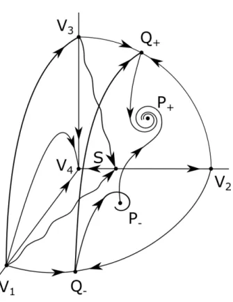
117
with one resident and one mutant phenotype. In this case, evolutionary
118
substitution and evolutionary replacement are equivalent since the question
119
in both cases is whether the mutant phenotype becomes established in the
120
system and the resident phenotype goes extinct.
121
The resident system of Lotka-Volterra type is of the form
122
˙
ρ1 =ρ1 r1+mRR11 ρ1
(1) where ρ1 is the resident density, r1 is the intrinsic growth rate and mRR11 is
123
the interaction parameter. Clearly, this system has a stable equilibrium with
124
ρ∗1 > 0 (i.e. with the resident species present) if and only if the intrinsic
125
growth is positive and the interaction term is negative (in which case, the
126
equilibrium is ρ∗1 =−r1/mRR11 ).2
127
We assume that the difference between resident and mutant behavior is
128
contained in the interaction parameters (e.g. the parameter mRI11 models the
129
linear effect that the mutant densityµ1has on the growth rate of the resident
130
2The notation used here is consistent with the more complicated LV systems in the remainder of the paper (e.g. (3) below) . It can be considerably simplified in this special case. For instance, with r1=r >0 and mRR11 =m <0, (1) is the logistic equation (i.e.
positive intrinsic growth and negative density dependence) in more standard notation.
phenotype).3 The corresponding resident-mutant system is then
131
˙
ρ1 =ρ1 r1+mRR11 ρ1+mRI11µ1
˙
µ1 =µ1 r1+mIR11ρ1+mII11µ1
. (2) If this models competition (i.e. all four interaction parameters are negative),
132
it is well-known (Hofbauer and Sigmund, 1998) that the two-dimensional
133
dynamical system evolves to the mutant equilibrium µ∗1 = −r1/mII11 if and
134
only if the mutant can invade the resident equilibrium but the resident cannot
135
invade the mutant equilibrium.
136
We say that general LV systems of the form (2) exhibit evolutionary sub-
137
stitution if (i) the one-dimensional resident system and mutant system respec-
138
tively each have a stable equilibrium with positive density; (ii) the resident
139
(respectively, mutant) equilibrium is unstable (respectively, stable) since it
140
can be invaded by the mutant phenotype (respectively, cannot be invaded
141
by the resident phenotype) in the two-dimensional resident-mutant system
142
(2); and (iii) after the mutant successfully invades the resident, the system e-
143
volves to the mutant equilibrium. In fact, these two-dimensional LV systems
144
exhibit evolutionary substitution if and only if r1 > 0, mRR11 < 0, mII11 < 0
145
(i.e. the resident system and the mutant system each have a globally stable
146
equilibrium) and mIR11 ≥ mRR11 , mII11 ≥ mRI11 with strict inequality in at least
147
one of these two conditions.
148
As interpreted by Cressman and Garay (2003a),r1 >0, mRR11 <0, mII11 <0 are the ecological stability conditions and mII11 ≥ mRI11 with mIR11 > mRR11 if mII11 = mRI11 means that the mutant phenotype is an evolutionarily stable s- trategy (ESS). That is, in addition to ecological stability, we have evolution- ary stability of the mutant phenotype since it is an ESS of the evolutionary game given by the 2×2 payoff matrix (or interaction matrix)
mRR11 mRI11 mIR11 mII11
.
In game-theoretic terms (Apaloo, 2006), the final condition for evolutionary
149
substitution (i.e. mIR11 ≥mRR11 with mII11 > mRI11 if mIR11 =mRR11 ) is equivalent
150
3That is, the intrinsic growth rate is independent of species phenotype. The discussion here does not rely on this assumption. In fact, for the N−species systems of Sections 3 and 4, Theorems 1 to 4 do not depend on our assumption that, for each species k, the resident and mutant phenotypes have the same intrinsic growth rate rk. Moreover, the proofs of these results do not rely on this assumption either.
to the mutant phenotype being a neighborhood invader strategy (NIS) of
151
the resident phenotype (i.e. the mutant phenotype that is sufficiently rare
152
successfully invades the resident phenotype). Strategies that satisfy both the
153
ESS and NIS conditions for matrix games such as given by the 2×2 payoff
154
matrix above are known as ESNIS (Apaloo, 2006).
155
In summary, there is evolutionary substitution/replacement in a single-
156
species LV system if and only if
157
(i) there is ecological stability in the resident system and in the mutant
158
system
159
(ii) the resident phenotype cannot invade the mutant phenotype (i.e. the
160
mutant phenotype is an ESS of the interaction matrix for the resident-mutant
161
evolutionary game), and
162
(iii) the mutant phenotype can invade the resident phenotype (i.e. the
163
mutant phenotype is a NIS of the resident phenotype for this interaction
164
matrix).
165
3 Evolutionary Substitution in N −Species
166
In this section, we assume that the N−species resident system has one resi-
167
dent phenotype in each species and that there is a single mutant phenotype
168
in exactly one species (which, without loss of generality, we take as species
169
one). If rk and ρkrespectively are the intrinsic growth rate and resident phe-
170
notype density of species k and µ1 is the density of the mutant phenotype,
171
then the resident-mutant Lotka-Volterra system is
172
˙
ρk = ρk rk+
N
X
l=1
mRRkl ρl+mRIk1µ1
!
(3)
˙
µ1 = µ1 r1+
N
X
l=1
mIR1l ρl+mII11µ1
!
where k= 1, ..., N. In particular, for LV systems, the individual growth rate
173
of a given phenotype (e.g. ˙ρk/ρk) are linear functions of the densities of all
174
phenotypes present in the system.
175
One interpretation of theinteraction parameters mRRkl , mRIk1, mIR1l andmII11
176
adopts the payoff terminology of evolutionary game theory (Cressman and
177
Garay, 2003a). Then mRRkl (respectively, mRIk1) is the payoff to a resident
178
phenotype (or strategy) in species k when interacting with a resident pheno-
179
type in speciesl(respectively, the intruder or mutant phenotype).4 Similarly,
180
mIR1l andmII11 are payoffs to the mutant phenotype. That is, the superscripts
181
denote the phenotypes and the subscripts are the species in the interaction
182
where the first superscript and subscript specify the phenotype and species
183
of the individual receiving the payoff, respectively
184
The first requirement for evolutionary substitution is that this resident
185
system is stable in the absence of mutants. In particular, from the biological
186
perspective, this means that there is species coexistence in the residence
187
system. Mathematically, there is a locally asymptotically stable equilibrium
188
ρ∗ = (ρ∗1, ..., ρ∗N) with all components positive (i.e. ρ∗ ∈RN>0) for the resident
189
system
190
˙
ρk =ρk rk+
N
X
l=1
mRRkl ρl
!
k= 1, ..., N. (4)
To avoid technical complications, we assume that this stability is determined
191
through the linearization of (4) about ρ∗. That is, we assume that the resi-
192
dent system is hyperbolic (i.e. all eigenvalues of the N ×N Jacobian matrix
193
of this linearization, which has kl entry ρ∗kmRRkl , have nonzero real parts).5
194
Thus this hyperbolic resident system is stable if and only if all eigenvalues
195
of the Jacobian matrix have negative real parts. Let MRR be the N ×N
196
matrix whose entries are the payoffs mRRkl for interactions between residents
197
(similarly, MIR denotes the 1×N matrix of payoffs to mutants interacting
198
with residents etc.). Then, in particular, MRR is invertible since its deter-
199
minant is non-zero and so ρ∗ = − MRR−1
r where r is the column vector
200
whose kth component is the intrinsic growth rate rk of species k.
201
The next requirement is that the mutant phenotype can invade. That
202
is, (ρ∗,0) is not a locally asymptotically stable equilibrium of the resident-
203
mutant system (3). (ρ∗,0) will be unstable in the resident-mutant system
204
if the invasion fitness λI1 ≡ r1 +PN
l=1mIR1l ρ∗l of the mutant phenotype at
205
4In evolutionary game theory, it is usually assumed that each individual has one random pairwise interaction per unit time. Here, the number of such interactions for an individual is proportional to the density in each species.
5The Jacobian matrix at the resident equilibrium ρ∗ is
ρ∗1 0 0 0 . .. 0
0 ρ∗N
MRR.
this equilibrium is greater than the fitness of the resident phenotype r1 +
206
PN
l=1mRR1l ρ∗l = 0 (i.e. if λI1 > 0). On the other hand, (ρ∗,0) is locally
207
asymptotically stable if λI1 <0. In the intermediate case where λI1 = 0, the
208
mutant phenotype is initially selectively neutral when invading the resident
209
equilibrium. This case was analyzed by Cressman and Garay (2003a, 2003b)
210
who showed that, for Lotka-Volterra systems, (ρ∗,0) is invadable if and only
211
if MII −MIR MRR−1
MRI ≥0.
212
Finally, after successful invasion by the mutant, evolutionary substitution
213
requires that the resident-mutant system must evolve to a locally asymptot-
214
ically stable equilibrium (0,ρb2, ...,ρbN,µb1) with all species present but species
215
one has only mutant phenotypes. In particular, this equilibrium cannot be
216
invaded by the resident phenotype of species one. That is, the invasion fit-
217
ness of the resident phenotype of species one, λR1 ≡r1+PN
l=2mRR1l ρbl+mRI11µb1
218
cannot be positive at (0,ρb2, ...,ρbN,µb1).6
219
The question arises whether hyperbolic stability of ρ∗ and (ρb2, ...,ρbN,bµ1)
220
in their respective N− dimensional Lotka-Volterra systems (which we as-
221
sume from now on) implies evolutionary substitution if the mutant phenotype
222
can invade (ρ∗,0) but the resident phenotype of species one cannot invade
223
(0,ρb2, ...,ρbN,µb1). Such an implication would generalize the evolutionary sub-
224
stitution in a single species discussed in Section 2. Our first result (Theorem
225
1) implies that a unique coexistence equilibrium is impossible in this case.
226
Theorem 1 Suppose that E1 ≡(ρ∗,0) and E2 ≡(0,ρb2, ...,ρbN,µb1) are equi-
227
libria of theN-species resident-mutant LV system (3) with all species present
228
(i.e. ρ∗i >0 for i= 1,2, ..., N and ρbj >0 for j = 2, ..., N and µb1 >0). Also
229
assume that E1 and E2 are locally asymptotically stable equilibria for system
230
(3) restricted to their respective N−dimensional boundary face and that the
231
mutant phenotype can invade E1 but the resident phenotype of species one
232
cannot invade E2.7 Then there is no isolated interior equilibrium8 for the
233
N + 1 dimensional LV system.
234
Proof. Letx∗ = (x∗1, x∗2, ..., x∗N, x∗N+1) be an isolated interior equilibrium
6In the threshold case when the resident phenotype is initially selectively neutral (i.e.
λR1 = 0), the analogue of MII −MIR MRR−1
MRI must now be negative (see the B-matrix method of Cressman and Garay (2003a)).
7Under these assumptions, we say that the invasion conditions are satisfied.
8That is, every neigborhood of an equilibrium with all N + 1 components positive contains another equilibrium.
for (3), which for convenience, we rewrite as
˙
xi =xi ri+
N+1
X
j=1
aijxj
!
for i= 1,2, ..., N + 1.
The isolatedness assumption implies that the (N + 1)×(N + 1) interaction
235
matrix Awith entriesaij is invertible. An application of Cramer’s Rule (see,
236
for instance the proof of Theorem 13.5.7 in Hofbauer and Sigmund (1998))
237
shows that
238
x∗i =−|Ai |
|A| ri+ (Axi)i
(5) whenever the principal submatrixAi ofA formed by deleting theith row and
239
column is nonsingular and, apart from thei-th coordinate which is then taken
240
as xii = 0, the remaining coordinates of xi = (xi1, . . . , xii−1,0, xii+1, . . . , xiN+1)
241
are defined as the coordinates of the unique solution to the linear system
242
rj + (Ax)j = 0 for allj 6=i.
243
From the assumptions in the statement of the theorem, x1 (respectively, xN+1) is the equilibriumE2 (respectively, E1). Sincex1 andxN+1 are locally asymptotically stable in their respective N−dimensional boundary faces, A1 andAN+1are both nonsingularN×N matrices and their determinants|A1 | and | AN+1 | have the same sign. Moreover, since the mutant phenotype can invade the resident equilibrium, rN+1+ (AxN+1)N+1 ≥ 0 and since the resident phenotype cannot invade the mutant equilibrium, r1+ (Ax1)1 ≤0.
Thus
x∗1x∗N+1 = |A1 ||AN+1 |
|A|2 r1+ (Ax1)1
rN+1+ (AxN+1)N+1
≤0 which contradicts that x∗ is an interior equilibrium.
244
Remark 1. The proof of Theorem 1 above relies on the nonsingularity
245
of A. For general A, (5) can be rewritten as
246
|A|x∗i =− |Ai | ri+ (Axi)i
. (6) In fact, this reformulation holds whenever Ai is nonsingular for any solution
247
x∗ of Ax+r = 0 (see the proof in Appendix A1).9 Thus, if A is singular,
248
9The first and fourth authors refer to this general result as the Calgary Lemma, the location where they obtained its proof that has as yet been unpublished as far as they are aware.
then (ri+ (Axi)i) = 0 whenever Ai is nonsingular (in particular, for i = 1
249
and i=N+ 1). That is,λI1 = 0 = λR1. In this case,Ax1+r= 0 =AxN+1+r
250
and so the line segment joining E2 = x1 and E1 = xN+1 are all equilibria
251
of the system (3). In particular, E2 is not locally asymptotically stable in
252
the extended, (N + 1)−dimensional phase space since there are arbitrarily
253
close initial points on this line segment that do not evolve to it (i.e. it can be
254
invaded by the resident phenotype of species one). Thus, the conclusion of
255
Theorem 1 can be strengthened to show that there is no interior equilibrium
256
for the N + 1 dimensional LV system when the invasion conditions hold.
257
For evolutionary substitution to occur, it is necessary that no interior
258
equilibrium exists. However, the converse is not true. That is, evolutionary
259
substitution is not guaranteed when there is no interior equilibrium as the
260
following two-species example illustrates. In particular, ecological stability
261
together with the invasion conditions of Theorem 1 do not imply evolutionary
262
substitution unlike the single-species result of Section 2.
263
Example 1 Consider the resident-mutant three-dimensional LV system
264
˙
ρ1 = ρ1(−4−3ρ1+ 7ρ2−4µ1)
˙
ρ2 = ρ2(−1−ρ1+ 2ρ2−µ1) (7)
˙
µ1 = µ1(−4 + 7ρ2−3µ1).
It is readily checked that the conditions of Theorem 1 are satisfied for
265
N = 2, equilibria E1 = (ρ∗1, ρ∗2,0) = (1,1,0), E2 = (0,ρb2,bµ1) = (0,1,1) and
266
λI1 =−4 + 7 = 3>0, λR1 =−4 + 7−4 =−1<0. The equilibria of (7) are
267
the origin O = (0,0,0), P+ =E2 (which are asymptotically stable10) and the
268
saddle points P− =E1 and S= (0,12,0).
269
The global dynamics of (7) as well as the dynamics of the resident sub-
270
system
271
˙
ρ1 =ρ1(−4−3ρ1 + 7ρ2)
˙
ρ2 =ρ2(−1−ρ1+ 2ρ2) (8)
10Since 0< ρ2<12 implies ˙ρ2<0 and thus ˙ρ2<−12ρ2<0 as well as ˙µ1<−12µ1<0 , the origin attracts all points of the open, unbounded 3D rectangle 0< ρ1<∞, 0< ρ2<12, 0< µ1<∞. The region of attraction of the origin is separated from the rest of the phase portrait by (the non-negative part of) the two-dimensional, unbounded stable manifold of the saddle pointS.
and of the mutant subsystem
272
˙
µ1 =µ1(−4−3µ1+ 7ρ2)
˙
ρ2 =ρ2(−1−µ1+ 2ρ2):, (9)
are presented in Figure 1. The three thick gray curves portray nonplanar
273
trajectories, including the outgoing trajectory of P−. Due to lack of space,
274
ingoing and outgoing trajectories of the saddle point S are not shown but
275
clearly indicated by trajectories nearby. All black trajectory curves are planar.
276
Orientation of the trajectories is determined by the stability properties of the
277
equilibria. The behavior of the trajectories far from the origin is nontrivial
278
and presented in Figure 2 of Appendix A2.
279
When ρ1 in (8) is changed to µ1 in (9), it is immediate that the dynamics
280
in the µ1-ρ2 plane is exactly the same as in the ρ1-ρ2 plane. Please observe
281
this symmetry in both Figures.
282
Figure 1: Phase portrait of the replicator system (7).
[ROSS: Please check that footnote 10 is placed where Barnabas intended
283
it and that the figure is okay. The difference between the gray and black
284
curves is not that great. Maybe the gray ones could be some other color
285
(red?) instead? I have inserted the sentence on orientation into the text
286
since figure 1 does not have arrows on the trajectories.]
287
By Example 1, the invasion criteria of Theorem 1 do not imply evolution-
288
ary substitution for two-species LV systems. On the other hand, if the LV
289
system has more structure, the invasion criteria of Theorem 1 can be equiv-
290
alent to evolutionary substitution. The following discusses two such systems
291
of biological importance.
292
First, for two-species competitive LV systems, evolutionary substitution
293
is equivalent to the invasion criteria. These resident-mutant systems have
294
the form
295
˙
xi =xi ri+
3
X
j=1
aijxj
!
for :i= 1,2,3 (10) where r1 = r3 and r2 are all positive and aij < 0 for i, j = 1,2,3. By the
296
discussion above, the invasion criteria are necessary for evolutionary substi-
297
tution. The following theorem proves the converse. In fact, for such systems,
298
the invasion criteria imply that E2 = (0,ρb2,bµ1) is globally asymptotically
299
stable.
300
Theorem 2 Suppose that E1 ≡ (ρ∗1, ρ∗2,0) and E2 ≡ (0,ρb2,µb1) are equilib-
301
ria of the two-species resident-mutant competitive LV system (10) with both
302
species present (i.e. ρ∗i > 0 for i = 1,2, ρb2 > 0 and µb1 > 0) and satisfying
303
r1 = r3 > 0, r2 > 0 and aij < 0 for i, j = 1,2,3. Also assume that E1
304
and E2 are locally asymptotically stable equilibria for system (10) restricted
305
to their respective two-dimensional boundary face. If the mutant phenotype
306
can invade E1 but the resident phenotype of species one cannot invade E2,
307
then E2 is globally asymptotically stable.11
308
Proof. It is well-known (e.g. Zeeman, 1993) that the dynamic behavior of
309
anN+1−dimensional competitive LV system is determined by its restriction
310
to an invariantN−dimensional hypersurface called the carrying simplex (van
311
den Driessche and Zeeman, 1998). For the three-dimensional system (10),
312
the two-dimensional carrying simplex in the first octant is homeomorphic to
313
a triangle whose three edges correspond to boundary invariant curves of (10)
314
11Here, and everywhere else in the present paper, both for LV and replicator systems, global asymptotic stability (gas) of an equilibrium means that it is locally asymptotically stable (las) and attracts all interior trajectories. Similarly, “gas restricted to a face” means
“las restricted to this face and attracts all interior trajectories on this face”.
whose endpoints are the carrying capacities −ri/aii of the logistic equation
315
for each species i on its own.
316
By Theorem 1 and Remark 1, (10) has no interior equilibria. Moreover,
317
E1 ≡(ρ∗1, ρ∗2,0) corresponds to a saddle point on the x1x2 edge whose stable
318
manifold is this edge andE2 ≡(0,ρb2,µb1) corresponds to a stable equilibrium
319
on thex2x3 edge of the triangle. Thus, of the 33 possible classes of dynamic
320
behavior classified by Zeeman (1993), the dynamics on the triangle is given
321
by one of classes 9 to 12 depending on the behavior on the x1x3 edge. In all
322
four classes, the equilibrium corresponding to E2 is globally asymptotically
323
stable.
324
Evolutionary substitution also occurs when the mutant phenotype “dom-
325
inates” the resident phenotype it substitutes for according to the following
326
theorem. Here, dominance is used in the game-theoretic sense in that the
327
expected payoff (or fitness) of an individual using the mutant phenotype is
328
greater than that of the resident phenotype (i.e. the mutant is more fit)
329
whenever some phenotypes are present (see (11) below).
330
Theorem 3 As in Theorem 1, let E1 ≡ (ρ∗,0) and E2 ≡ (0,ρb2, ...,ρbN,bµ1)
331
be equilibria of the N-species resident-mutant LV system (3) with all species
332
present (i.e. ρ∗i > 0 for i = 1,2, ..., N and ρbj > 0 for j = 2, ..., N and
333
µb1 >0). Furthermore, assume that all forward trajectories of (3) are bound-
334
ed12 and that E2 is globally asymptotically stable equilibrium for system (3)
335
restricted to its N−dimensional boundary face. If the mutant phenotype is
336
always more fit than the resident phenotype of species one, then there is no
337
interior equilibrium, the resident phenotype of species one goes extinct and
338
E2 is a locally asymptotically stable equilibrium for system (3). Moreover,
339
if no interior trajectories converge to the boundary of the N−dimensional
340
boundary face containing E2, then evolutionary substitution occurs.
341
Proof. Since the mutant phenotype is always more fit than the resident
342
phenotype of species one
343
r1+
N
X
l=1
mIR1l ρl+mII11µ1 > r1+
N
X
l=1
mRR1l ρl+mRI11µ1 (11)
12That is, each trajectory is defined for allt≥0 and all its components are less thatD for some D >0 that may depend on the trajectory.
for all (ρ1, ρ2, ..., ρN, µ1) with nonnegative components and at least one com-
344
ponent positive. In particular, this inequality holds atE1 andE2 (i.e. λI1 >0
345
and λR1 <0). Since λR1 <0 and E2 is globally asymptotically stable equilib-
346
rium for system (3) restricted to its N−dimensional boundary face, E2 is a
347
locally asymptotically stable equilibrium for system (3).
348
The resident phenotype of species one goes extinct if every interior tra-
349
jectory of (3) converges to the N−dimensional boundary face with ρ1 = 0.
350
Actually, this convergence holds for every trajectory with ρ1 and µ1 initially
351
both positive. To see this, consider a given trajectory with ρ1 andµ1 initial-
352
ly positive. The first and the last equation of system (3) yield that dtd µρ1
1
353
equals
354
ρ1µ1
r1+PN
l=1mRR1l ρl+mRI11µ1
−ρ1µ1
r1+PN
l=1mIR1l ρl+mII11µ1 µ21
= −ρ1
µ1 r1+
N
X
l=1
mIR1l ρl+mII11µ1
− r1+
N
X
l=1
mRR1l ρl+mRI11µ1
!
<0 for all (ρ1, ρ2, ..., ρN, µ1) where ρ1 and µ1 are both positive. The final in-
355
equality follows from (11). Thus, ρµ1
1 is a strictly decreasing function a-
356
long every trajectory where ρ1 and µ1 are initially both positive. For the
357
given interior trajectory, define limt→∞ ρ1(t)
µ1(t) = C ≥ 0. If C = 0, then
358
limt→∞ρ1(t) = 0 since µ1(t) is bounded. Suppose that ρ1 does not converge
359
to 0 (i.e. lim supt→∞ρ1(t) >0). Thus, C > 0 and there exists a limit point
360
of the given trajectory with ρ1 and µ1 both positive. Any trajectory that
361
is initially at this limit point is also in the limit set of the given trajectory.
362
Since µρ1
1 is a strictly decreasing at this initial point, limt→∞ ρ1(t)
µ1(t) < C, a
363
contradiction. Since the resident phenotype ρ1 goes extinct, there can be no
364
interior equilibrium.
365
As a by-product of the previous considerations, we see that interior trajec-
366
tories converge to nonempty compact subsets of the N−dimensional bound-
367
ary face ρ1 = 0 of the non-negative (N+ 1)−dimensional orthant. This is the
368
boundary face that contains equilibrium E2. By the last assumption of the
369
theorem, interior trajectories have a limit point with the properties ρ1 = 0
370
and ρ2ρ3. . . ρNµ1 >0. Since E2 is globally asymptotically stable for system
371
(3) restricted to the face ρ1 = 0 and locally asymptotically stable for the full
372
resident-intruder system (3) on RN+1≥0 , E2 is the only limit point of any given
373
interior trajectory. That is, interior trajectories converge to E2. In other
374
words, evolutionary substitution occurs.
375
Remark 2. The condition in Theorem 3 thatE2is globally asymptotical-
376
ly stable equilibria for system (3) restricted to its N−dimensional boundary
377
face is necessary for the conclusion that evolutionary substitution occurs. To
378
see this, consider Example 1 again. In it, we have that the mutant fitness
379
−4 + 7ρ2 −3µ1 is always greater than the fitness −4−3ρ1 + 7ρ2 −4µ1 of
380
the resident phenotype of species one when ρ1 and µ1 are positive. However,
381
evolutionary substitution does not occur in Example 1 since (0,0,0) is local-
382
ly asymptotically stable. Note that Theorem 3 also makes the biologically
383
reasonable assumption that the density of each species must be bounded.
384
4 Evolutionary Replacement
385
In this section, we assume that the N−species system has one resident phe-
386
notype and one mutant phenotype in each species. Then the resident-mutant
387
Lotka-Volterra system is
388
˙
ρk = ρk rk+
N
X
l=1
mRRkl ρl+mRIkl µl
!
(12)
˙
µk = µk rk+
N
X
l=1
mIRkl ρl+mIIklµl
!
where MII, MRI, MIR, MRR are now all N ×N interaction matrices.
389
The first requirement of evolutionary replacement is that the invasion
390
criteria for system (12) be satisfied. That is, the N−dimensional resident
391
system has a locally asymptotically stable interior equilibrium E1 ≡ (ρ∗,0)
392
(where ρ∗i >0 fori = 1,2, ..., N) that can be invaded by the mutant pheno-
393
types and the N−dimensional mutant system has a locally asymptotically
394
stable interior equilibriumE2 ≡(0, µ∗) (whereµ∗i >0 fori= 1,2, ..., N) that
395
cannot be invaded by the resident phenotypes. The following example shows
396
that these invasion conditions do not rule out the existence of a stable interior
397
equilibrium of the resident-mutant system. Thus, the obvious generalization
398
of Theorem 1 is not valid for evolutionary replacement.
399
We then examine extensions of the domination concept of Theorem 3 to
400
replacement systems. In this section, we concentrate on examples with two
401
species (i.e. N = 2) since Example 1 shows that care must already be taken
402
when there are two species and a single mutant phenotype.
403
Example 2 Consider the resident-mutant system
404
˙
ρ1 = ρ1(2−ρ1 −µ1)
˙
ρ2 = ρ2(3−ρ2 −2µ1)
˙
µ1 = µ1(2−2ρ1+ρ2−µ1)
˙
µ2 = µ2(3−3ρ1+ρ2−µ2).
The intrinsic growth rates of species one and two are r1 = 2 and r2 = 3
405
respectively. This has an interior equilibrium at (ρ1, ρ2, µ1, µ2) = (1,1,1,1)
406
that is locally asymptotically stable since the only eigenvalue of the corre-
407
sponding 4×4 Jacobian matrix is −1 (with multiplicity 4). The resident
408
system has a globally asymptotically stable equilibrium at (ρ∗1, ρ∗2) = (2,3)
409
and the mutant system also has a globally asymptotically stable equilibrium
410
at (µ∗1, µ∗2) = (2,3). Moreover, to analyze whether (ρ∗1, ρ∗2)can be invaded, we
411
calculate λI1 = 2−2ρ∗1+ρ∗2 = 1>0 andλI2 = 3−3ρ∗1+ρ∗2 = 0. Similarly, to
412
analyze whether (µ∗1, µ∗1) can be invaded, we calculate λR1 = 2−µ∗1 = 0 and
413
λR2 = 3−2µ∗1 =−1<0.
414
Since the eigenvalue λI2 is zero (respectively, λR1 = 0), it is not imme-
415
diately clear whether (ρ∗1, ρ∗2,0,0) = (2,3,0,0) (respectively, (0,0, µ∗1, µ∗2) =
416
(0,0,2,3)) can be invaded. To avoid the use of B-matrix methods for these
417
neutral invasion coefficients (Cressman and Garay, 2003a), we consider in-
418
stead the slightly perturbed system
419
˙
ρ1 = ρ1(2−ρ1−(1 +ε)µ1)
˙
ρ2 = ρ2(3−ρ2−2µ1) (13)
˙
µ1 = µ1(2−2ρ1+ρ2−µ1)
˙
µ2 = µ2(3−3ρ1+ (1 +ε)ρ2−µ2) with some ε > 0. The new interior equilibrium
1−5ε
1−2ε,1−6ε1−2ε,1−2ε1 ,1+4ε−6ε1−2ε 2
420
will still be locally asymptotically stable when ε is sufficiently small. More-
421
over, the equilibrium of the resident system remains unchanged at(ρ∗1, ρ∗2,0,0) =
422
(2,3,0,0)as does the equilibrium for the mutant system(0,0, µ∗1, µ∗2) = (0,0,2,3).
423