Effect of metasomatism on the electrical resistivity of the lithospheric mantle – An integrated research using magnetotelluric sounding and xenoliths beneath the N ´ ogr ´ ad-G om ¨ or Volcanic Field ¨

(1)

Global and Planetary Change 197 (2021) 103389

Available online 4 December 2020

(http://creativecommons.org/licenses/by-nc-nd/4.0/).

Effect of metasomatism on the electrical resistivity of the lithospheric mantle – An integrated research using magnetotelluric sounding and xenoliths beneath the N ´ ogr ´ ad-G om ¨ or Volcanic Field ¨

Levente Patk o ´

^a^,^b^,^c^,^d

, Attila Nov ´ ak

^b^,^d

, Rita Kl ´ ebesz

^d

, N ´ ora Liptai

^b

, Thomas Pieter Lange

^a^,^b

, G abor Moln ´ ´ ar

^d^,^e

, L ´ aszl ´ o Csontos

^f

, Viktor Wesztergom

^b^,^d

, Istv ´ an J ´ anos Kov ´ acs

^b^,^d

,

Csaba Szab o ´

^a^,^d^,^*

aLithosphere Fluid Research Lab (LRG), E¨otv¨os Lor´and University, Budapest, Hungary

bLendület Pannon LitH2Oscope Research Group, Research Centre for Astronomy and Earth Sciences (CSFK), Sopron, Hungary

cIsotope Climatology and Environmental Research Centre, Institute for Nuclear Research (ATOMKI), Debrecen, Hungary

dGeodetic and Geophysical Institute, Research Centre for Astronomy and Earth Sciences (CSFK), Sopron, Hungary

eGeological, Geophysical and Space Research Group of the Hungarian Academy of Sciences, E¨otv¨os Lor´and University, Budapest, Hungary

fExploration & Production Division, MOL Group, Budapest, Hungary

A R T I C L E I N F O Keywords:

Long period magnetotellurics Upper mantle xenoliths Low electrical resistivity Mantle metasomatism Wehrlitization

A B S T R A C T

Long period magnetotelluric (MT) data were collected at 14 locations along a ~50 km long NNW-SSE profile in the Nógrád-Gömör Volcanic Field (NGVF), which is one of the five mantle xenolith bearing Neogene alkali basalt locations in the Carpathian-Pannonian region. As a result, a low resistivity anomaly (<10 Ωm) was observed approximately at 30–60 km depth beneath the central part of the NGVF, indicating the presence of a conductive body beneath the Moho. This is the same area where upper mantle xenoliths with wehrlitic modal composition were collected from six quarries. The wehrlites were formed as a result of mantle metasomatism involving the peridotite wall rock and a mafic melt. The spatial coincidence of the geophysical anomaly and the petrographic- geochemical alteration in the upper mantle suggests their probable relationship. To test this assumption, we estimated the electrical resistivity of the wehrlites. The outcome reveals lower electrical resistivity for wehrlites (~132 Ωm) compared to the non-metasomatized lherzolites (~273 Ωm) from the same localities. However, it is still higher than the values acquired with long period MT soundings. Thus, further modelling was implemented in order to test the possible role of melt. The models revealed that even ~2–3 vol.% of interconnected melt is enough to lower the electrical resistivity below 1 Ωm in the wehrlites. The interconnected glass phase found in the wehrlites may be the evidence for this later solidified melt. All these suggest that melts may still be present in small amounts beneath the cooling NGVF. The intensive melt upwelling in the central part of the NGVF resulting in a wehrlitized mantle portion with low electrical resistivity, as well as the extensive basalt flows on the surface, can be explained by deep deformation zones, which provide excellent migration pathways for melts through the entire lithosphere.

1. Introduction

Magnetotellurics (MT) is routinely used both in the industrial and academic research. In mineral, hydrocarbon and geothermal explora- tions, audio-MT studies are applied mostly for shallow crustal (i.e.

250–2000 m) depths (e.g. Strangway et al., 1973; Aiken and Ander, 1981; Orange, 1989). In academic studies, MT is usually used for addressing a specific geological problem and the investigated depth

usually ranges from a few tens of kilometers up to ~200 km. These studies aim to define compositions, structures and processes in the crust and in the upper mantle (Hautot et al., 2000; Selway et al., 2009; Muller et al., 2009; Bologna et al., 2011; Ad´ ´am et al., 2017; Evans et al., 2019).

MT is especially sensitive to detect partial melts/fluids by quantifying resistivity (Wannamaker et al., 2002; Hill et al., 2009; Becken and Ritter, 2012; Selway et al., 2019), and it is commonly applied to detect the lithosphere–asthenosphere boundary (LAB) or other surfaces in the

* Corresponding author.

E-mail address: cszabo@elte.hu (C. Szab´o).

Contents lists available at ScienceDirect

Global and Planetary Change

journal homepage: www.elsevier.com/locate/gloplacha

https://doi.org/10.1016/j.gloplacha.2020.103389

Received 15 May 2020; Received in revised form 20 November 2020; Accepted 21 November 2020

(2)

mantle characterized by changes in electrical resistivity due to physico- chemical changes (e.g. Praus et al., 1990; Eaton et al., 2009; Jones et al., 2010). Even though the resolution of MT deep sounding becomes gradually worse with increasing depth and measurements can be challenging due to the presence of shallow, slightly resistive layers, good resolution can be achieved even at great depths (>30 km) with careful planning of station density and adequate data processing. Furthermore, several case studies show that far more information can be extracted by combining electrical models with petrologic data than only considering the resistivity distribution within the studied volume (Khan et al., 2006;

Fullea et al., 2011; Jones et al., 2012; Voz´ar et al., 2014).

In this paper, we investigated whether the assumed lithological heterogeneities and/or the presence of melt/fluid in the lithospheric mantle beneath the Nógrád-Gömör Volcanic Field (NGVF) (Fig. 1) can be studied by MT. The NGVF is the northernmost of the five, mantle xenolith-bearing alkali basalt volcanic fields in the Carpathian- Pannonian region (CPR) (Fig. 1a). The spatial distribution of the xenoliths and their petrographic and geochemical characteristics are well known (Szabó and Taylor, 1994; Liptai et al., 2017; Patkó et al., 2020a).

The dominant lithology in the mantle is lherzolite (~75% of all xenoliths), however, the large number of wehrlite xenoliths (~20% of all xenoliths) and the detailed geochemical study of the lherzolite xenoliths indicate that the upper mantle beneath the NGVF was affected by several metasomatic events, the last of which caused the formation of the wehrlites (Liptai et al., 2017; Patk´o et al., 2020a). However, xenoliths are only fragments of the lithospheric mantle and the spatial distribution of this metasomatized mantle domain is unknown. Thus, the goal of this study was to image the lithospheric mantle of the NGVF, map the LAB, and determine whether the distribution of the lithological differences can be constrained by MT. We provide a geological interpretation for the MT data obtained along a profile across the study area (Fig. 1b), using theoretical calculations to compare the electrical resistivity with compositional differences of the peridotite. In the electrical resistivity modelling, the presence of melt/fluid is also taken into account. This case study of combined geological and geophysical methods may help interpreting deep MT results worldwide, even where mantle xenolith data are not available. Our research delivers information on the root zone of an intraplate volcanic field, where the magmatism may be more extensive and longer lasting even after the latest active eruptions than it was previously thought based only on the areal extent and volume of erupted products.

2. Geological settings

The Pannonian Basin is situated in East-Central Europe surrounded by the Alpine, Carpathian and Dinaric orogenic chains (Fig. 1a). It consists of two tectonic megaunits, ALCAPA in the northwest with Mediterranean affinity and Tisza-Dacia in the southeast with dominantly European origin, which are divided by the Middle Hungarian Shear zone (Stegena et al., 1975; Balla, 1984; Kázmér and Kovács, 1985;

Fodor et al., 1999; Csontos and Vor¨¨os, 2004). The NGVF is located at the northern edge of the Pannonian Basin (Fig. 1a) on the ALCAPA mega- unit. The Gemeric and Veporic sub-units (in fact Alpine nappes within ALCAPA) comprise the basement of the NGVF, consisting mostly of Paleozoic and Mesozoic sequences, and sheared and tectonized crystalline nappes (Tomek, 1993; Koroknai et al., 2001). In the cover sequence, there are Tertiary sediments and volcanic rocks such as Miocene andesites and Plio-Pleistocene alkali basalts and their pyro- clasts (Fig. 1b). The alkali basalt products of the NGVF consist of maars, diatremes, tuff cones, cinder/spatter cones and lava flows, which are dispersed in an area of ~150 km²(Koneˇcný et al., 1995a). The formation of alkali basalts is related to post-extensional thermal relaxation of the asthenosphere, which is the source of these melts as a result of small degree partial melting (<5%) (Embey-Isztin et al., 1993; Harangi, 2001;

Lexa et al., 2010). It has been recently proposed that compression in the tectonic inversion stage of the CPR evolution may have squeezed partial

Fig. 1.(a) Simplified geological map of the Carpathian-Pannonian region (CPR) with the inferred ALCAPA–Tisza-Dacia microplate boundary (after Csontos and Nagymarosy, 1998 and references therein). Xenolith-bearing Neogene alkali basalt volcanic fields shown are the following: SBVF - Styrian Basin Volcanic Field; LHPVF - Little Hungarian Plain Volcanic Field; BBHVF - Bakony–Balaton Highland Volcanic Field; NGVF - Nógrád-Gömör Volcanic Field; PMVF - Perșani Mountains Volcanic Field. (b) Simplified geological map of the Nógrád-Gom¨ ör Volcanic Field (modified after Hok et al. (2014) and Lexa ´ et al. (2000)) with the position of xenolith sampling localities (black star) and magnetotelluric stations (red circle). Xenolith sampling quarries from NW to SE are the following: Podreˇcany (NPY), Maˇsková (NMS), Jelˇsovec (NJS), Trebe- l’ovce (NTB), Fil’akovské Kova´ˇce (NFK), Fil’akovo-Kerˇcik (NFL), Ratka (NFR), Maˇcacia (NMC), Magyarbánya (NMM), Eresztvény (NME) and Bárna-Nagyk˝o (NBN). (For interpretation of the references to color in this figure legend, the reader is referred to the web version of this article.)

(3)

melt out from the asthenosphere (Kov´acs et al., 2020).

The volcanic activity in the NGVF took place between 6.17–1.35 Ma based on K-Ar dating (Balogh et al., 1981). New results of combined U/

Pb and (U–Th)/He geochronometry (Hurai et al., 2013) have slightly extended the period of volcanism (7–0.3 Ma). Mantle xenoliths are abundant in the alkali basalt at NGVF from Podreˇcany (NPY) in the northwest to Bárna (NBN) in the southeast (Fig. 1b), however they are absent in the mafic volcanics east of Fil’akovo. These mantle xenoliths have variable compositions, with samples belonging to the Cr-diopside (Hovorka and Fejdi, 1980; Szabó and Taylor, 1994; Koneˇcný et al., 1995b; Liptai et al., 2017; Patko et al., 2020a) and Al-augite (Kov´ ács

et al., 2004; Zajacz et al., 2007) series defined by Wilshire and Shervais (1975). Among the Cr-diopside rocks, a lherzolitic and wehrlitic series were distinguished (Liptai et al., 2017; Patk´o et al., 2020a), the latter only present in the central outcrops NGVF (Babi Hill and Medves Plateau; Fig. 1b).

3. Method

Magnetotellurics (MT) is based on the ultra and extremely low frequency (ULF-ELF) geomagnetic field time variation and its response to the conductive Earth according to the Faraday law of induction

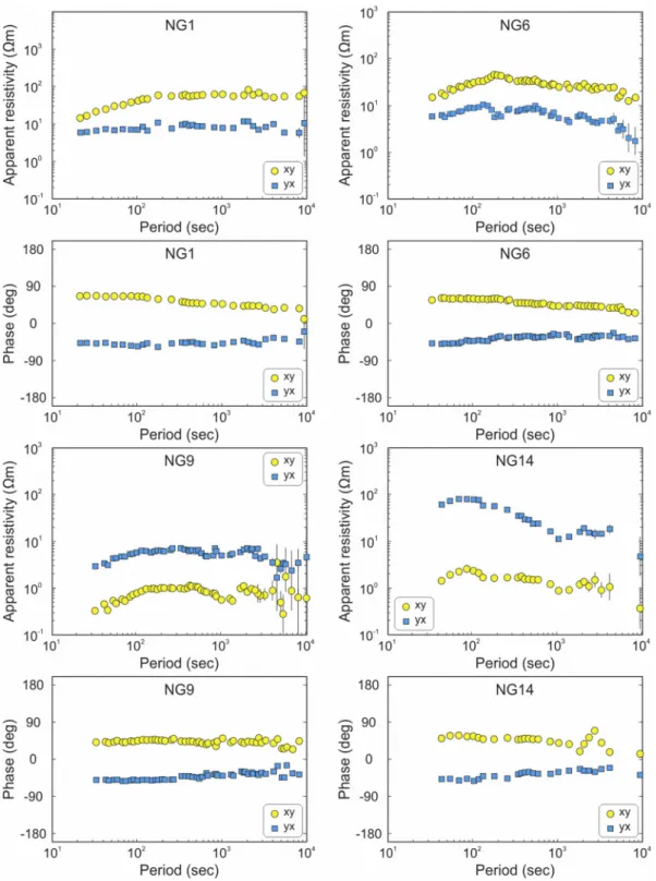
Fig. 2. Characteristic raw magnetotelluric sounding curves of apparent resistivities and impedance phases at four selected sites: NG1, NG6, NG9, NG14.

(4)

(Tikhonov, 1950; Cagniard, 1953). The penetration depth of the electromagnetic (EM) waves depends on the period and resistivity of ma- terials. The EM field observed on the surface is the superposition of primary (ionospheric, magnetospheric current system) and secondary (subsurface induction) sources. The induction effect (i.e. EM properties of the subsurface) is detectable on the surface in the form of impedance tensor, which is the frequency dependent transfer function of the electric and magnetic field vectors. The complex elements of the impedance tensor are parameters that provide information on geoelectrical structures. These parameters are the following: apparent resistivity (bulk average resistivity), phase of the impedance; geomagnetic transfer function (induction vector) and dimension indicators (e.g. phase tensor ellipses) which are derived from primary impedances (Wiese, 1962;

Swift, 1967; Bibby, 1977; Caldwell et al., 2004; Berdichevsky and Dmitriev, 2010).

During 2013 to 2014, long period MT data were collected at 14 stations (coordinates are listed in Supplementary Table 1) along a ~60 km long NNW–SSE profile in the NGVF (Fig. 1b) with the aim of char- acterizing the electrical resistivity image of the lithosphere and determining the depth of the LAB. During the measurements, a LEMI-417 acquisition system was applied, in which the time variation of the magnetic field components (Hx, Hy and Hz) were measured by flux-gate magnetometer. The telluric field components Ex and Ey were observed by non-polarized Cu-CuSO4 electrodes using 50 m long electric dipoles.

The orientation of the magnetic and telluric sensors was set to principal axis of Earth’s magnetic field (NS and EW). The distance between MT stations was 3–5 km depending on topography, location of xenolith- bearing quarries and potential man-made noise areas. In order to elim- inate artificial electromagnetic (EM) noise, three instruments were applied simultaneously, which allowed the implementation of remote

Fig. 3. (a) Rose diagrams of electrical strike directions for crustal (10–30 km), lithospheric mantle (30–70 km) and asthenospheric (70–120 km) depths. (b) Induction vectors and phase tensor ellipses for all MT stations (showing black arrows) at different time periods at estimated depths of 20, 30 and 40 km, respectively. Depth estimations are based on the averages of different approaches including Skin depth (Cagniard, 1953), Bostick depth (Bostick and Smith, 1962), modified Bostick depth (Martí i Castells, 2006) and Schmucker depth (Schmucker, 1973).

(5)

reference approach (Varentsov et al., 2003). The average recording time was approximately 4–5 days at a single station. The electromagnetic time variations were collected at a rate of 4 Hz, where the available period range was approximately between 10 and 10000 s. The time series were processed using robust single-site, and in two cases (NG12 and NG13 stations; Fig. 1b), remote reference processing code to estimate MT transfer functions (Egbert and Booker, 1986; Egbert and Livelybrooks, 1996). Strong artificial electromagnetic noise was observed in case of some MT stations (NG9, NG11, NG12; Fig. 1b), which were situated in the vicinity of settlements. Occasionally, telluric wires were damaged by animals, which restricted the length of the appropriate time series. In order to reach the LAB depth and construct broadband MT sounding curves, the recorded effective EM time variation lasted minimum 36 h without any disturbances. Selected MT sounding curves are shown on Fig. 2. The transfer function of the MT stations was estimated using on average 48 frequency bands and 0.95 coherency condition for electric and magnetic field components.

4. Electrical strike directions, induction vectors and phase tensor ellipses

Before the 1-D and 2-D inversions, we calculated the electrical strike directions, induction vectors and phase tensor ellipses too.

The electrical strike directions were calculated by tensor decomposition following the method of Groom and Bailey (1989). The results were grouped by 3–4 MT stations and illustrated on rose diagrams (Fig. 3a). The calculated directions point predominantly to NNE (Fig. 3a). Significant variation was only observed in the group of NG4- NG7 stations, where the crust shows N44^◦E, whereas the mantle has around N10^◦E–N15^◦E electrical strike. In the northern part of the MT profile (NG12–NG14), minimal diversity was observed in the electrical strike of different depth ranges (N23^◦E–N26^◦E) (Fig. 3a). The estab- lished geoelectric strike direction is N20^◦E.

Induction vectors were calculated from geomagnetic data based on the considerations of Wiese (1962). The induction vectors provide information on the position and extent of potential low resistivity (<10 Ωm) bodies. The length of the induction vector defines the electrical resistivity, whereas its direction points towards the low electrical resistivity anomalies. At periods between 43–341 s (~20–50 km), the induction vectors of some MT stations located at central and northern part of the profile (NG8–NG14) point to the south and have great length (Fig. 3b). The long vectors disappear at greater depth (>50 km), and their direction changes dominantly to SE and NE at ~60 km and ~100 km, respectively (Fig. 3b).

The magnetotelluric phase tensor ellipse (Caldwell et al., 2004) is a tool to obtain information on the dimensionality of the regional electrical structures by galvanic distortion. It is defined by the inverse tangent ratio between the imaginary and real parts of the magnetotelluric tensor (Weaver et al., 2000). The phase tensor ellipses refer to the dimension of electrical structures by ellipticity and β skew angle (represented by colors) of the ellipses. In the northern part of the profile (NG10–NG14), phase tensor ellipses have strong ellipticity and high β skew angle (>0) for periods 43–341 s (Fig. 3b). In the same MT stations, the ellipticity remains strong, but the β skew angles turn to a negative value at periods 512–1365 s. In MT stations NG4–NG9, the phase tensor ellipses are moderately variable, whereas those at the southernmost three MT stations (NG1–NG3) are quite homogenous for the entire section (Fig. 3b).

5. 1-D and 2-D inversion results

Reduction of the MT data was carried out using different inversion models including layered 1-D (Geosystem, 2000), automatic Occam’s 1- D (Constable et al., 1987) and 2-D inversions (Rodi and Mackie, 2001).

The static shift and galvanic distortion were eliminated by Groom-Bailey decomposition (Groom and Bailey, 1989). Both the layered and the

automatic Occam’s 1-D inversions (Fig. 4a) were calculated applying the invariant apparent resistivity.

The layered 1-D inversion gives the electrical resistivity and thick- ness of layers in all MT stations (Fig. 4a). The appropriateness of the inversion was verified by the low RMS (root mean square) misfit value (average RMS =0.1355) (Supplementary Fig. 1). The presented values are in nRMS (normalized RMS). The layers south of the NG12 station are characterized by low electrical resistivities (<20 Ωm) (Fig. 4a). The only exception is the depth range of ~10–25 km, where electrical resistivity values are dominantly over 40 Ωm (Fig. 4a). In the northern part of the MT profile (NG12–NG14), high electrical resistivity values (>100 Ωm) are the most frequent (Fig. 4a). For determining the asthenospheric indication, only those layers were taken into account where the electrical resistivity dropped by 5–25 Ωm below 50 km. According to these criteria, the LAB depth is placed between 54–70 km south of the NG12 station (Fig. 4a; Table 1). Further asthenospheric indication was observed beneath the three northernmost stations (NG12–NG14) with an estimated LAB depth of >100 km (Table 1; Supplementary Fig. 1).

Based on the automatic Occam’s 1-D inversion results (Fig. 4a), the electrical resistivity is uniformly low (<10 Ωm) in the upper part of the crust (top 5 km). Beneath the central part of the section (NG9-NG10 stations) an anomaly with low electrical resistivity (<10 Ωm) was detected at lower crustal depth (10–20 km). In contrast, beneath the southern and the northern part of the section, highly resistive bodies (>500 Ωm) were found in the lower crust. The rest of the lower crust has an average of ~100 Ωm electrical resistivity. Below the crust, a conductive anomaly was detected with a low resistivity (<5 Ωm) at

~20–60 km depth range in the central part of the section (NG6–NG11 stations) (Fig. 4a). The horizontal extension of this anomaly is more than 30 km. The indication of the asthenosphere at 60–80 km depth is observed in the southern 30 km of the section (Fig. 4a). However, in the rest of the section, the depth of the LAB was impossible to determine (Fig. 4a).

In order to test the results of the 1-D inversions, we carried out 2-D inversion as well. The sounding curves (Fig. 2) were rotated with N20^◦E based on the electrical strike direction (Fig. 3a). The 2-D inversion was inverted by the non-linear conjugate gradient algorithm of Rodi and Mackie (2001) implemented in WinGLink software. In the modelling, homogeneous half-space approach was applied with 100 Ωm electrical resistivity as an average value based on the result of the 1-D inversion (Fig. 4a). The elevation of the stations was also taken into account. In order to achieve the final 2-D model, a few tests (>10) were carried out to obtain the best smoothing parameters of error floor, electrical resistivity range, regularization parameter, static shift correction and weighting function. The 2-D inversions were carried out using bimodal inversion (Transversal Electric (TE) +Transversal Mag- netic (TM)), where the conjugate data of the vertical magnetic compo- nent (Hz) was taken into account. Error floor of 5% for both TE and TM modes were applied. The static shift correction was automatically used and the RMS was minimized by 100 iterations. Data errors were set to 10% (apparent resistivity) and 5% (phase) (Supplementary Fig. 2). For equal weighting of apparent resistivity and phase in the inversion, the error of phase was selected as the half of that for apparent resistivity.

Error floors of apparent resistivity and phase were both 5%, where phase error is introduced in % equivalent to apparent resistivity error (i.e., 1%

apparent resistivity error is equivalent to a 0.29 degree absolute error in phase). The error floor for induction vector was set to 0.1 absolute magnitude value. Since the average amplitude of induction vector magnitude is ~0.6 and the standard deviation is ~0.3, we determined the error floor values to be 0.1 (~15%). The Supplementary Fig. 3 shows the fitting of the induction vectors in 2-D inversion.

The best solution of the inversion is shown on Fig. 4b. The shallow part of the section (<20 km) shows several elongated (5–10 km) anomalies with high (>100 Ωm) and low (<10 Ωm) resistivity values (Fig. 4b). Below the Moho a low resistivity (<2 Ωm) structure has been revealed in the depth range of 30–60 km beneath stations NG5-NG9

(6)

(Fig. 4b), with a horizontal extension of ~15 km. In the southern part of the section (beneath stations NG1–NG9), indication of the asthenosphere with low electrical resistivity (~1 Ωm) appears at the depth of

~80 km (Fig. 4b).

6. Expected electrical resistivity in the lithospheric mantle We carried out estimations on the electrical resistivity of the rock forming mantle silicates (olivine, orthopyroxene, clinopyroxene) and calculated bulk rocks. As first approach, the effect of fluids/melts were avoided, and only the solid wall rock was considered. We used the excel worksheet modified after Kovacs et al. (2018) (Supplementary Table 2) ´ for the calculations. This estimation follows the methodology specified in Fullea (2017). We applied the first parameterization (PC1) (Fullea, 2017 and references therein) in the third term of the equation describing the conductivity of mantle minerals (Supplementary Table 2). Further details are described in Kov´acs et al. (2018).

In order to calculate the electrical resistivity values for NGVF xenoliths, the characteristic petrographic and geochemical data of the local mantle are needed in addition to the experimentally derived parameters (e.g., activation enthalpies, pre-exponential terms). The ‘water’ content of the nominally anhydrous minerals (NAMs), which refers to hydrogen incorporated in the crystal lattice as hydroxyl and commonly expressed as H2O, is probably the most important factor in electrical resistivity (Wang et al., 2006; Dai and Karato, 2009; Yoshino et al., 2009; Poe et al., 2010; Yang et al., 2011; Novella et al., 2017). The clinopyroxene, orthopyroxene and olivine have ‘water’ contents in a decreasing amount in mantle (Bell and Rossman, 1992; Ingrin and Skogby, 2000; Demouchy Fig. 4. (a) Layered 1-D (columns) and automatic Occam’s 1-D inversion models of the MT profile. (b) 2-D inversion model of the MT profile. The static shift and galvanic distortion were eliminated by Groom-Bailey decomposition (Groom and Bailey, 1989). The Moho depth is based on Horv´ath et al. (2006) and Kl´ebesz et al. (2015).

Table 1

List of the MT stations, with the estimated depth of lithosphere-asthenosphere boundary (LAB) using the 1- D layered inversion (Geosystem, 2000). In some stations (NG1, NG7, NG8, NG10, NG11) results were invalid and are thus not shown. Results of the NG13 and NG14 MT stations are unrealistic and were not taken into account.

MT station LAB depth (km)

NG1 –

NG2 70

NG3 67

NG4 61

NG5 68

NG6 67

NG7 –

NG8 –

NG9 54

NG10 –

NG11 –

NG12 106

NG13 169

NG14 159

(7)

and Bolfan-Casanova, 2016; Peslier et al., 2017).

In the NGVF, clinopyroxenes have lower ‘water’ content (0.5–481 with an average of 132 ppm) in lherzolites than in the strongly metasomatized wehrlites (21–894 with an average of 302 ppm) (Patk´o et al., 2019). Among clinopyroxenes in wehrlite xenoliths, dry (21–464 with an average of 140 ppm) and wet (202–894 with an average of 481 ppm) grain populations were distinguished based on their water ‘contents’ (Patko et al., 2019). The ‘water´ ’ content of the orthopyroxenes is variable in lherzolites (1–147 with an average of 31 ppm) (Patk´o et al., 2019). Note that ‘water’ data of orthopyroxenes is not available for wehrlites and certain lherzolites. The ‘water’ content of the lherzolitic olivines is usually below detection limit. Similarly, there is no detectable

‘water in wehrlitic olivines either (Patk´o et al., 2019). The low ‘water’

content of NAMs is most likely because of pre-, syn- and post-entrapment hydrogen loss (Patk´o et al., 2019). The reason why clinopyroxene was affected the least and olivine the most is the different hydrogen diffusion speed in these minerals (e.g. Tian et al., 2017 and references therein). In xenoliths where the ‘water’ data of orthopyroxene or olivine was not detected, we made estimations on the original hydrogen concentration.

Thus, the analyzed ‘water’ content of clinopyroxenes together with the partition coefficient of hydrogen between clinopyroxene and other silicates were applied (D^cpx/opx=2.3; Pint´er et al., 2015; D^cpx/ol=10; Xia et al., 2019). Sometimes the estimated ‘water’ contents for olivines resulted in higher values than concentrations measured in orthopyroxenes, which is unrealistic. Thus, in such cases the ‘water’ content of the orthopyroxenes was calculated as well from clinopyroxene data. All measured and calculated ‘water’ contents are listed in Supplementary Table 3.

Modal compositions, the XFe (XFe =1 − Mg#/100) ratio of the silicates and equilibration temperatures are taken from Liptai et al. (2017) and Patk´o et al. (2020a) for lherzolites and wehrlites, respectively (Supplementary Table 3). The pressure at the origin of the xenoliths is hard to estimate for spinel facies xenoliths. The best approach is to use the alkaline basalt province geotherm (Jones et al., 1983) and the equilibration temperatures (based on the Ca-in-opx thermometer of Nimis and Grütter (2010) modified after the thermometer of Brey and K¨ohler (1990); TCa-in-opx by NG10), which allows an estimation for the pressure (Supplementary Table 3).

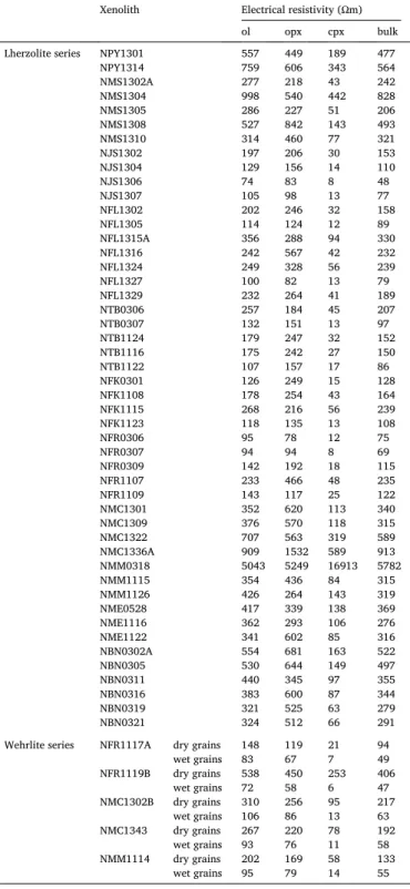
The calculated electrical resistivity values are listed in Table 2. We omitted lherzolite NMM0318 because of its extremely high electrical resistivity (>5000 Ωm for all silicates, respectively) most likely due to its extremely low ‘water’ concentration (Supplementary Table 3). The calculated electrical resistivity has similarly wide ranges in lherzolitic olivines (74–998 with an average of 314 Ωm) and orthopyroxenes (78–1532 with an average of 364 Ωm) (Fig. 5a). In contrast, the electrical resistivity of clinopyroxenes in lherzolites has a narrower range with lower values (8–589 with an average of 92 Ωm). We calculated the electrical resistivity of the wet and the dry grains of wehrlites separately (Table 2). The electrical resistivity in the order of decreasing values is the following in wet grains: olivine (72–106 with an average of 90 Ωm), orthopyroxene (58–86 with an average of 73 Ωm) and clinopyroxene (6–14 with an average of 10 Ωm) (Fig. 5a). The same values are higher in dry grains: olivine (148–538 with an average of 293 Ωm), orthopyroxene (119–450 with an average of 243 Ωm) and clinopyroxene (21–253 with an average of 101 Ωm) (Fig. 5a). The bulk rock electrical resistivity is higher in lherzolites (48–913 with an average of 273 Ωm) compared to that in wehrlites calculated using dry (94–406 with an average of 208 Ωm) and wet grains (47–63 with an average of 55 Ωm) (Fig. 5b). In case of the lherzolite bulk rock, electrical resistivities are different based on spatial distribution. There are high average electrical resistivities in the northern (NPY–520 Ωm; NMS–418 Ωm) as well as in the southern- central (NMC–539 Ωm; NMM–317 Ωm; NME–320 Ωm) and southern (NBN–381 Ωm) NGVF localities (Fig. 1b). The only exception is Jelˇsovec locality in the north (NJS–97 Ωm), which has low average electrical resistivity likewise in the northern-central sites (NFL–188 Ωm;

NTB–138 Ωm; NFK–160 Ωm; NFR–123 Ωm) (Fig. 1b).

7. Discussion

7.1. Geological interpretation of MT data 7.1.1. Crust

Even though the position of the Moho cannot be detected by MT (Fig. 4), it is reasonable to divide and interpret the observed structures based on their location relative to the known Moho. The crustal thick- ness beneath the study area is well constrained, the Moho stretches at 25–30 km in depth (Horv´ath et al., 2006; Kl´ebesz et al., 2015).

The northern part of the profile (NG12–NG14 stations) is situated on a terrain where the Veporicum outcrops on the surface (Fig. 1b), therefore the resistive (45–150 Ωm) layers that appear both in 1-D and 2-D inversion models were interpreted to represent the metamorphic complexes of the Veporicum crystalline units (Fig. 4). Comparing our results with the MT data obtained along nearby profiles (Bez´ak et al., 2014, 2015, 2020), it is reasonable to assume that this resistive body is part of the Veporic granitoid complex.

In the southern and central parts of the profile (NG1–NG11 stations), the crust is characterized by relatively low electrical resistivity structures (<80 Ωm) on 1-D inversion image (Fig. 4a). The shallow, less resistive (<10 Ωm) structures are associated with Neogene to Quater- nary sediments underlain by Eocene to Early Miocene sedimentary rocks and possibly Gemeric metasediments containing graphitic shales (Bez´ak et al., 2015 and references therein). The deeper parts of the crust are likely composed of Veporic crystalline rocks, i.e. sub-thrust of the Gemerides (Bez´ak et al., 2015), which are also known in several bore- holes in adjacent areas (Koroknai et al., 2001). However, the resolution of the sounding is not enough to differentiate among Veporic units.

Between stations NG9 and NG10, (and below stations NG2 to NG8 to some extent,) the body with low electrical resistivity (<10 Ωm) may be physically and/or genetically connected to the low resistivity crustal structures observed in the 2T profile of Bez´ak et al., 2015. The authors interpreted these structures to be the result of prior intensive Neogene tectonic and volcanic processes associated with conductive fluid migration and hydrothermal ore mineralization.

The 2-D inversion results (Fig. 4b) reveal several low (<10 Ωm) and high (>100 Ωm) resistivity bodies in the crustal level of the southern and central parts of the profile (NG1–NG11 stations). This higher resolution of 2-D than 1-D inversions for the crust is due to the application of TE+TM modes and geomagnetic data (Hz). The heterogeneous crust and the lack of drilling cores also make the interpretation of the MT data challenging. The low resistivity anomaly found beneath the NG9 and NG10 MT stations is also observed on the 2-D inversion image, with lateral extension stretching below stations NG8-NG6 (Fig. 4b). The previously described interpretation of fluid migration linking to tectonic and volcanic processes (Bez´ak et al., 2015) can be feasible here as well.

The electrical strike directions and phase tensor ellipses in crustal depth can be also explained by local crustal geology. Electrical strike directions are varying between N4^◦E–N44^◦E (Fig. 3a). This is roughly perpendicular to the SW-NE strike direction of tectonic unit boundaries in the Carpathian thrust system (e.g. Plaˇsienka et al., 1997). The reason of the strong ellipticities and high β skew angles in the northern part of the profile is attributed to the presence of Veporic units with 3D electrical structures (Fig. 3b).

7.1.2. Lithospheric mantle

The sub-Moho part of the profile is characterized by similar electrical resistivity distribution both on 1-D and 2-D inversion images (Fig. 4).

Generally, the lithospheric mantle has electrical resistivity <100 Ωm.

The only exception is below the two northwestern most stations (NG13–NG14), where the high electrical resistivity (>100 Ωm) determined for the crust extends towards the lithospheric mantle as well (Fig. 4). These two stations are located north of the surface appearance of the alkali basaltic volcanic products (Fig. 1b). Thus, it is reasonable to deduce that the generally higher electrical resistivity in the lithospheric

(8)

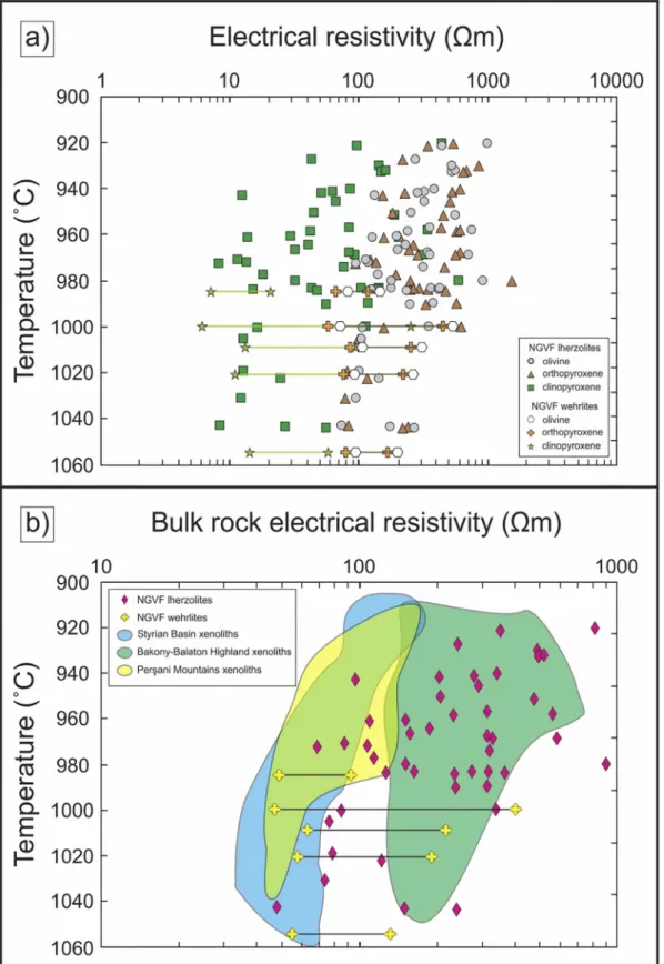
Fig. 5. (a) Electrical resistivity of the rock forming minerals (olivine, clinopyroxene, orthopyroxene) of N´ogr´ad-Gom¨ or lherzolite and wehrlite xenoliths in function ¨ of equilibration temperature. The results of dry and wet wehrlitic grains from the same xenoliths are connected with solid lines showing wet grains by lower electrical resistivity values. (b) Bulk rock electrical resistivities of lherzolite and wehrlite xenoliths in function of equilibration temperature. Reference data were calculated based on Aradi et al. (2017) for Styrian Basin, Liptai et al. (2021) for Bakony-Balaton Highland and Falus et al. (2008) and Lange et al. (2019) for Pers¸ani Mountains.

The results of the same wehrlites using dry and wet grains, respectively, are connected with solid lines showing wet grains by lower electrical resistivity values.

(9)

mantle under these stations is related to the lacking effect of volcanism on the mantle. The melt migration in association with the alkali basaltic volcanic activity may have pervasively metasomatized mantle volumes along the melt migration pathways and decreased the electrical resistivity. The extension of Veporic granitoid units below the local Moho as an explanation for high electrical resistivity is definitely less likely.

Beneath the central part of the NGVF, directly below Moho, a low resistivity body (<10 Ωm) appears both in 1-D and 2-D inversion images (Fig. 4). The anomaly extends till the depth of ~60 km (Fig. 4), which is also supported by the disappearing long induction vectors at greater depths (Fig. 3b). The spatial distribution of wehrlite xenoliths correlates well with this observed anomaly (Patko et al., 2020a). To answer the ´ question whether wehrlite bodies can be the reason for the anomaly, the results of electrical resistivity calculations can be examined and compared with those of the lherzolites, which represent the precursor mantle rocks of the wehrlites (Patk´o et al., 2020a).

7.1.2.1. Low resistivity anomaly in the mirror of wehrlite and lherzolite characteristics. The electrical resistivity of a peridotite depends on several factors. Numerous studies in the past two decades revealed that the greater the ‘water’ content of nominally anhydrous minerals (NAMs), the lower their electrical resistivity (Wang et al., 2006; Dai and Karato, 2009; Yoshino et al., 2009; Poe et al., 2010; Yang et al., 2011;

Jones et al., 2012; Novella et al., 2017). The presence of wet clinopyroxenes with high ‘water’ contents (>202 ppm) in the NGVF wehrlites causes high ‘water’ concentrations in the bulk rock (>62 ppm), resulting in wehrlites having lower electrical resistivity than ‘dryer’ wall rock lherzolites (Patkó et al., 2019). Other factors like modal composition, geochemical characteristics and pressure-temperature conditions all have an impact on the electrical resistivity, but their effect is less significant (Selway, 2014; Fullea, 2017). According to Karato and Wang (2013), the electrical resistivity of NAMs is the following in decreasing order: olivine, orthopyroxene, clinopyroxene, which is true for the NGVF as well (Fig. 5a). It follows that the elevated clinopyroxene content in wehrlites (~21 vol.%; Patkó et al., 2020a) compared to the lherzolites (~9 vol.%; Liptai et al., 2017) results in lower bulk electrical resistivity. The greater iron concentration in the mineral phases, and consequently in bulk rocks, leads to lower electrical resistivity as well (Hinze et al., 1981; Seifert et al., 1982; Omura et al., 1989; Yoshino et al., 2012). Since the wehrlitization leads to Fe enrichment, wehrlites have higher Fe contents than lherzolites (Patko et al., 2020a). According ´ to experiments conducted with multi-anvil apparatus, increasing pressure and temperature considerably reduces the electrical resistivity in olivines (Xu et al., 2000; Yoshino et al., 2012), whereas in pyroxenes, this effect is minimal (Dai et al., 2006). There is a small difference in the pressure-temperature conditions of the NGVF wehrlites (985–1055 with an average of 1014 ^◦C using TCa-in-opx by NG10 and 1.3–1.6 GPa; Patkó et al., 2020a) and lherzolites (921–1044 with an average of 973 ^◦C using TCa-in-opx by NG10 and 1.2–1.5 GPa; Liptai et al., 2017), which may have a weak additional role in the lower electrical resistivity of the former.

As a conclusion, all parameters suggest lower electrical resistivity in wehrlite than in lherzolite xenoliths. Therefore, the wehrlitization must have considerable effect on the electrical resistivity in the mantle volume affected by metasomatism. This is further supported by the estimated electrical resistivity of bulk rocks, which are lower for wehrlites (average values are 55 and 208 Ωm based on wet and dry grains, respectively) than lherzolites (with an average of 273 Ωm) (Table 2).

Although the modal proportion of wet and dry rock forming minerals is unknown in the wehrlites, their bulk electrical resistivity is likely no higher than 150 Ωm.

Note that electrical resistivity difference exists not only between the wehrlite and the lherzolites xenolith, but also appears among the lherzolite samples. The northern-central localities (NFL, NTB, NFK, NFR;

Fig. 1b) are characterized with lower average electrical resistivities (<200 Ωm; Table 2). Similarly, the northern locality of Jelˇsovec has low Table 2

Electrical resistivity results of the rock forming silicates and bulk rocks of the Nógrád-Gom¨ or wehrlite xenoliths. The values were calculated using the excel ¨ worksheet of Supplementary Table 2 modified after Kovács et al. (2018). Ab- breviations: ol - olivine, opx - orthopyroxene, cpx - clinopyroxene, bulk - calculated whole rock.

Xenolith Electrical resistivity (Ωm)

ol opx cpx bulk

Lherzolite series NPY1301 557 449 189 477

NPY1314 759 606 343 564

NMS1302A 277 218 43 242

NMS1304 998 540 442 828

NMS1305 286 227 51 206

NMS1308 527 842 143 493

NMS1310 314 460 77 321

NJS1302 197 206 30 153

NJS1304 129 156 14 110

NJS1306 74 83 8 48

NJS1307 105 98 13 77

NFL1302 202 246 32 158

NFL1305 114 124 12 89

NFL1315A 356 288 94 330

NFL1316 242 567 42 232

NFL1324 249 328 56 239

NFL1327 100 82 13 79

NFL1329 232 264 41 189

NTB0306 257 184 45 207

NTB0307 132 151 13 97

NTB1124 179 247 32 152

NTB1116 175 242 27 150

NTB1122 107 157 17 86

NFK0301 126 249 15 128

NFK1108 178 254 43 164

NFK1115 268 216 56 239

NFK1123 118 135 13 108

NFR0306 95 78 12 75

NFR0307 94 94 8 69

NFR0309 142 192 18 115

NFR1107 233 466 48 235

NFR1109 143 117 25 122

NMC1301 352 620 113 340

NMC1309 376 570 118 315

NMC1322 707 563 319 589

NMC1336A 909 1532 589 913

NMM0318 5043 5249 16913 5782

NMM1115 354 436 84 315

NMM1126 426 264 143 319

NME0528 417 339 138 369

NME1116 362 293 106 276

NME1122 341 602 85 316

NBN0302A 554 681 163 522

NBN0305 530 644 149 497

NBN0311 440 345 97 355

NBN0316 383 600 87 344

NBN0319 321 525 63 279

NBN0321 324 512 66 291

Wehrlite series NFR1117A dry grains 148 119 21 94

wet grains 83 67 7 49

NFR1119B dry grains 538 450 253 406

NMC1302B dry grains 310 256 95 217

wet grains 106 86 13 63

NMC1343 dry grains 267 220 78 192

NMM1114 dry grains 202 169 58 133

(10)

average electrical resistivity (NJS–97 Ωm). In contrast, the rest of the localities (NPY, NMS, NMC, NMM, NME, NBN; Fig. 1b) all have higher average electrical resistivities (>300 Ωm; Table 2). This can be explained by the ‘water’ content variability in the lherzolites (Supple- mentary Table 3). Jelˇsovec is the only locality, where the xenoliths are in pyroclastic rocks, so their higher ‘water’ content is possibly related to their fast cooling on surface (Patko et al., 2019). Note however that ´ water concentrations are only conservative estimates, even in Jelˇsovec locality, because ‘water’ loss cannot be excluded. Therefore, electrical resistivity values are maximum estimates, which can be lower.

7.1.2.2. Possible role of fluids/melts in low electrical resistivity. The estimated electrical resistivity of wehrlites is lower than those of the lherzolites (Fig. 5b), however, not as low as measured by MT (Fig. 4). Thus, the metasomatic alteration solely cannot account for the observed anomaly. Graphite films on grain boundaries (Mareschal et al., 1995;

Glover, 1996; Santos et al., 2002; Jones et al., 2003) or the presence of interconnected fluids/melt (Desissa et al., 2013; Johnson et al., 2016;

Ebinger et al., 2017; Magee et al., 2018; Selway et al., 2019, 2020) can further decrease the electrical resistivity, and may clarify the observed discrepancy. Graphite was not found in the studied xenoliths, hence its effect on lowering the electrical resistivity is unlikely. In contrast, the presence of fluids and melts are proved by fluid (Koneˇcn´a, 1990; Szabo ´ and Bodnar, 1996, 1998) and silicate melt inclusion (Szab´o et al., 1996;

Patk´o et al., 2018; Liptai et al., 2020) studies. Furthermore, the wehrlite (Patko et al., 2020a) and cumulate formation (Kov´ ´acs et al., 2004;

Zajacz et al., 2007) suggest intense fluid and melt migration, especially beneath the central part of the NGVF.

A recent study (Patk´o et al., 2020b), on volumetric ratio and spatial distribution of solid phases and vesicles in metasomatized wehrlites from NGVF using X-ray microtomography revealed presence of 2–6 vol.

% glass with no relationship to the host basalt, forming an interconnected network along grain boundaries. The glass is accompanied by 0.4–1.5 vol.% of vesicles, which represents pores after the loss of formerly dissolved gas phases (Patk´o et al., 2020b). This suggests that at the time of the entrapment of xenoliths in the host basalt, silicate melt was present in the upper mantle, which solidified into glass due to cooling most likely on the surface. The last phase of alkali basalt volcanism in the NGVF ceased about 0.3 Ma ago in the central part of the NGVF (Hurai et al., 2013). Since the longevity of such systems may span on the magnitude of 100 ka (Bourdon et al., 1994), some fluids or melts may still exist in the upper mantle beneath the central NGVF, which can lead to a decrease in the electrical resistivity. Note that experimental runs reveal that even ~0.5 vol.% of basaltic melt can form interconnected network and thus lower the electrical resistivity (Laumonier et al., 2017). The potential presence of melts beneath NGVF coincides with the implication of Kovacs et al. (2020), who concluded that partial ´ melts could be still present in the asthenosphere of CPR and can infil- trate to the lithospheric mantle along deep deformation zones.

If we accept the assumption that partial melt could still pond underneath the NGVF, a question raises regarding its amount. To answer this question, a numerical modelling was carried out based on the methodology in Sifr´e et al. (2014). Note that estimated electrical resistivity of dry and wet wehrlites (Table 2) as input parameter of melt- free metasomatic products was used. We examined the effect of increasing amount of melt (0–10 vol.%) containing various quantities of dissolved CO2 (0–2 wt.%) on electrical resistivity. The H2O content of the melt was calculated for each wehrlite xenolith using the bulk ‘water’ content of the wehrlites (Supplementary Table 4) and the partition coefficient of H2O between silicate melt and the mineral constituents (olivine, orthopyroxene, clinopyroxene) according to the formulae of Hirschmann et al. (2009). The results reveal 0.01–0.2 wt.% and 0.2–0.5 wt.% water contents for silicate melts being in equilibrium with dry and wet wehrlites, respectively (Supplementary Table 4). The detailed description of the modelling can be found in Supplementary Text 1.

The results of the modelling show similar images irrespectively to the different starting wehrlites (Fig. 6). The major inference is that the higher the melt fraction in the peridotite, the lower the electrical resistivity. The only exception is a field characterized by melt fraction greater than ~1 vol.%, accompanied with low CO₂content (<0.6 wt.%).

In case of small melt fraction (<1 vol.%), the amount of CO2 in the melt does not influence the electrical resistivity. In contrast, when the melt fraction exceeds 1 vol.%, the higher the CO2 content in the melt, the lower the electrical resistivity.

The X-ray microtomography done by Patko et al. (2020b) revealed ´ 2–6 vol.% interconnected glass in wehrlites in the NGVF. This suggests that the melt fraction reasonable to consider is equal to this range. The CO2 concentration of the melt can also be constrained with the use of silicate melt inclusions (SMIs), which are representative melt drops.

According to Szab´o et al. (1996), the CO₂content of SMIs has an average of 1.55 wt.%. Based on the study of Patko et al. (2020a), such inter-´ mediate melts can be formed during wehrlitization as a result of orthopyroxene dissolution. Similar average CO₂ concentration of wehrlitization related SMIs (1.68 wt.%) was calculated using the data of Liptai et al. (2020). On the modelled diagrams (Fig. 6), melt fractions of 2–5 vol.% and CO₂contents of 1.5–1.7 wt.% suggest electrical resistivities of <1 Ωm. It is likely that the 2–6 vol.% melt fraction was only valid for the interval of active volcanism, which could have ceased 300 ka ago (Hurai et al., 2013). Note however that even as little as 1 vol.% of melt can reduce the electrical resistivity to ~2.5 Ωm, and 0.5 vol.% melt fraction leads to ~5 Ωm electrical resistivity.

The conclusion drawn from the xenoliths and the electrical resistivity modelling is that the anomaly measured with MT is likely explained by wehrlite bodies with <2 vol.% interconnected silicate melt. Thus, it is reasonable to assume that the MT measurements reveal the distribution of wehrlitization. Based on this conclusion, the metasomatism affected a large volume of the mantle (~30 km long and ~15 km thick), which suggests that migration of the metasomatic melt along grain boundaries was quite extensive. In addition, it is plausible to assume that ponding, interconnected network of silicate melt is still present in the wehrlite- rich lithospheric mantle.

7.2. The depth of the lithosphere-asthenosphere boundary (LAB) Long period MT data are widely applied for LAB depth determination because of the contrast between the more resistive lithospheric mantle (generally few tens to hundreds Ωm) and the less resistive asthenosphere (generally 1–25 Ωm) (e.g. Korja, 2007). In this study, the depth of the LAB is defined by using the layered 1-D inversion model, however, the automatic Occam’s 1-D and the 2-D inversion models also suggest asthenospheric indications at somewhat greater depth (Fig. 4). Consid- ering that the research area is situated in the transition zone between the extended Pannonian Basin and the Carpathian orogen (Fig. 1a), a change in the depth of the LAB it is expectable. The result is ~65 km in the southern and central (NG2–NG11), and 105–170 km in the northern part (NG12–NG14) of the profile (Table 1; Supplementary Fig. 1). However, such an extreme variation in the LAB depth within a few tens of km is rather unlikely.

We compared our results with published LAB depth data implemented with various approaches. According to the review of Ad´ ´am and Wesztergom (2001), the LAB is located at a 75–85 km depth range beneath the NGVF based on MT measurements. Geissler et al. (2010) and Kl´ebesz et al. (2015) both used the receiver function approach and estimated a similar LAB depth, 74 km and 65 (±10) km, respectively.

The estimation of Taˇs´arov´a et al. (2009) using 3D gravity modeling reveal somewhat deeper LAB position (~80–100 km). An even thicker lithosphere of ~100–120 km was suggested by Bielik et al. (2010) using integrated 2D modeling of gravity, geoid, topography, and surface heat flow data.

Based on these results, the ~65 km and even the 106 km (Table 1) compares relatively well with literature. The reason we get ambiguous

(11)

results for some MT station regarding the LAB, especially from the central part of the NGVF (e.g. NG7, NG8, NG10, NG11; Table 1), can be the low resistivity body underneath this section of the MT profile (Fig. 4). The electric charges, which cause electromagnetic induction,

may be connected stronger to the conductive body located at shallower depths than the asthenospheric indication at greater depth (galvanic distortion effect; Chave and Smith, 1994).

The depths estimated beneath the northernmost stations Fig. 6. Modelled electrical resistivity of wehrlite xenoliths (NFR1117A, NFR1119B, NMC1302B, NMC1343, NMM1114) containing different amounts of melt (melt fraction) and variable dissolved CO2 concentrations. The boxes with dashed lines mark the field proposed for the NGVF (2–5 vol.% melt, 1.4–1.6 wt.% CO2). The possible melt fraction range is approximated by the modal presence of silicate glass in wehrlite xenoliths (Patko et al., 2020b), whereas the probable CO´ 2 content of the melt is defined by silicate melt inclusions from NGVF xenoliths (Szabo et al., 1996; Liptai et al., 2020). ´

(12)

(NG13–NG14 stations, >150 km) are significantly deeper than any published estimates. These data are unrealistic and likely caused by the shading effect of an extensive low resistivity body in the crust beneath these stations (Fig. 4). Such low resistivity anomaly can act as an insu- lator and cause uncertainty in determining electrical resistivity of greater depth below the anomaly.

As a conclusion, the LAB is at ~60–70 km and ~80–100 km in the southern and northern part of the MT section, respectively (Table 1).

This suggests a gradual LAB deepening towards the north.

7.3. Hurbanovo-Di´osjen˝o Line and its possible role in melt migration The 1-D and 2-D inversions reveal that the intensively metasomatized mantle volume is restricted to the central part of the NGVF (Fig. 4).

This is also the area, where long (>5 km) lava flows appear on surface in the form of Medves Plateau and Babi Hill (Fig. 1b). The question is raised, what can be the reason of this focused melt upwelling? Tectonic control is a possible explanation for this observation. The Hurbanovo- Diosjen´ ˝o Lineament and the Rapovce Fault is assumed to be located beneath the study area (Fig. 7), however, their exact position is uncer- tain. The WSW-ENE directed Hurbanovo-Di´osjeno Lineament represents ˝ a boundary between the highly-tectonized Central Western Carpathians and the barely deformed Transdanubian Range and Bükk units (Haas et al., 2014). The formation of this lineament started in Oligocene along with Paleogene basins in the northern CPR (Tari et al., 1993; Kov´aˇc et al., 2016). Further activities followed until the Pliocene-Quaternary boundary based on sedimentological interpretations (Kluˇciar et al.,

2016). The lineament is covered by several hundred meters thick Neogene to Quaternary sediments and volcanic rocks. Furthermore, the Hurbanovo-Diósjeno Lineament is not a discrete line but rather a few km ˝ wide dislocation zone (Balla, 1989). All these make the determination of the exact location challenging. Thus, borehole-based geological data (Balla, 1989) and geophysical methods such as geomagnetism (Haáz and Komáromy, 1967), gravity (Balla, 1989) and MT (Ad´ ám et al., 2003) were invoked earlier. Based on these, the lineament is assumed beneath the Medves Plateau (Fig. 1b).

To test this proposed location, the MT results can be of use. Tectonic zones are often characterized by low electrical resistivity values due to smaller average grain size (ten Grotenhuis et al., 2004) and presence of fluids/melts that migrate through (Brasse et al., 2002; Wannamaker et al., 2002). Furthermore, Pommier et al. (2018) revealed that tectonic zones are conduction paths in the shear direction. There are several low resistivity bodies (<10 Ωm) between the NG2–NG10 MT stations in the crust (<20 km depth) based on the 2-D inversion results (Fig. 4b). These MT stations cover the central part of the NGVF including the Medves Plateau and Babi Hill along a span of ~20–25 km (Fig. 1b). MT results beneath other part of the Hurbanovo-Di´osjen˝o Lineament 40–50 km to the west of the NGVF reveal similar low electrical resistivities (<20 Ωm) with lower crustal penetration depths (~15 km) (Ad´ ´am et al., 2003).

Therefore, this zone with low electrical resistivity values can be linked to diffuse tectonic structures, which confirms the presumption of Balla (1989) on a several km wide tectonic zone. Several faults including the Rapovce fault were distinguished by other MT studies targeted at the crust beneath the southern part of the Central Western Carpathians Fig. 6. (continued).

(13)

(Bez´ak et al., 2014, 2015, 2020). Comparing these prior sections with our measurements, the Rapovce fault is likely situated beneath the northern edge of the Babi Hill (Fig. 7) between stations NG9–NG10, where low resistivity zones in the crust appear according to the 2-D inversion model (Fig. 4b). Bez´ak et al. (2014, 2015, 2020) did not identify the Hurbanovo-Diosjen´ ˝o Lineament, which is to the south of the Rapovce fault and was likely out of the research area of those studies.

The Hurbanovo-Diósjen˝o Lineament may account for the low electrical resistivities beneath the Medves Plateau between stations NG4-NG5 (Fig. 4b). However, we cannot exclude that low electrical resistivities are linked to petrographic features. For example, graphitic shales and schists were found in some drilling cores reaching the Veporic and Gemeric units beneath the Cenozoic formations (K˝orossy, 2004). How-¨ ever, these wells aiming to reveal the hydrocarbon potential never reached depths greater than 2 km (Kor˝össy, 2004). According to Bezák et al. (2015), graphitic rocks are restricted to the shallower crust (<5 km), hence cannot be responsible for low electrical resistivity in the

lower crust.

Another question regarding the Hurbanovo-Di´osjen˝o dislocation zone and Rapovce fault is their possible penetration depths. According to the 2D-inversion image (Fig. 4b) beneath the NG2–NG10 MT stations, the low electrical resistivity zones are deep-rooted (reaching 20 km depth). This suggests that at least some of the fractures belonging to the dislocation zone reach the lower crust. Even more, these low resistivity volumes in the crust seem to be connected to the low resistivity anomaly situated beneath the Moho (Fig. 4).

This raises the possibility that these tectonic zones may crosscut not just the crust, but they extend even deeper in the lithospheric mantle. To investigate this possibility further, we summarized the results of previ- ous studies on deformation patterns of the NGVF upper mantle (Liptai et al., 2013, 2019; Klébesz et al., 2015). According to Liptai et al. (2019), most xenoliths have A-type orthorhombic crystal preferred orientation (CPO) symmetry in the central part of the NGVF, whereas it barely appears in the northern and southern parts. Orthorhombic CPO symmetry Fig. 7. Possible position of the Hurbanovo-Diósjeno Lineament and Rapovce fault in the NGVF based on the MT measurements and the conclusion of prior studies ˝ (Balla, 1989; Bezák et al., 2015, 2020).