Reduced-cost second-order algebraic-diagrammatic construction method for excitation energies and transition moments

Reduced-cost second-order algebraic-diagrammatic construction method for excitation energies and transition moments

Dávid Mester, Péter R. Nagy, and Mihály Kállay

Citation: The Journal of Chemical Physics 148, 094111 (2018); doi: 10.1063/1.5021832 View online: https://doi.org/10.1063/1.5021832

View Table of Contents: http://aip.scitation.org/toc/jcp/148/9 Published by the American Institute of Physics

Reduced-cost second-order algebraic-diagrammatic construction method for excitation energies and transition moments

D´avid Mester,^a)P´eter R. Nagy, and Mih´aly K´allay^b)

MTA-BME Lend¨ulet Quantum Chemistry Research Group, Department of Physical Chemistry and Materials Science, Budapest University of Technology and Economics, P.O. Box 91, H-1521 Budapest, Hungary

(Received 9 January 2018; accepted 19 February 2018; published online 7 March 2018)

A reduced-cost implementation of the second-order algebraic-diagrammatic construction [ADC(2)]

method is presented. We introduce approximations by restricting virtual natural orbitals and natural auxiliary functions, which results, on average, in more than an order of magnitude speedup com- pared to conventional, density-fitting ADC(2) algorithms. The present scheme is the successor of our previous approach [D. Mester, P. R. Nagy, and M. K´allay, J. Chem. Phys.146, 194102 (2017)], which has been successfully applied to obtain singlet excitation energies with the linear-response second-order coupled-cluster singles and doubles model. Here we report further methodological improvements and the extension of the method to compute singlet and triplet ADC(2) excita- tion energies and transition moments. The various approximations are carefully benchmarked, and conservative truncation thresholds are selected which guarantee errors much smaller than the intrin- sic error of the ADC(2) method. Using the canonical values as reference, we find that the mean absolute error for both singlet and triplet ADC(2) excitation energies is 0.02 eV, while that for oscillator strengths is 0.001 a.u. The rigorous cutoff parameters together with the significantly reduced operation count and storage requirements allow us to obtain accurate ADC(2) excita- tion energies and transition properties using triple-ζ basis sets for systems of up to one hundred atoms.Published by AIP Publishing.https://doi.org/10.1063/1.5021832

I. INTRODUCTION

There are several, nowadays, actively researched phenomena related to the excited electronic states of molec- ular systems. For instance, excited states play an impor- tant role for photochromic materials, for photo-initialized chemical processes, and for energy transfer and storage.

Quantum-chemical methods have now become routine tools in the investigation of excited-state properties and processes.

Consequently, it is important to develop efficient but reli- able methods for the excited states of extended molecular systems.

Many theories have been developed in the past few decades to investigate excited-state and transition properties.

These are, for example, the time-dependent density func- tional theory (TD-DFT)^1,2as well as the wave function-based semi-empirical^3–6andab initiomethods.^7–27Presently, for the investigation of extended systems with more than 1500 basis functions, a TD-DFT approach is the most common choice.

However, the limits of TD-DFT have been identified previ- ously for challenging cases,^28,29such as Rydberg and charge transfer (CT) states, or π → π^∗ excitations of a conju- gated system. The correlated wave function methods usu- ally provide a more reliable option for small cases. Excited states can simply be treated by the multi-configurational

a)Electronic mail: mester.david@mail.bme.hu

b)Electronic mail: kallay@mail.bme.hu

self-consistent field (MCSCF)³⁰ method, by the multi- reference configuration interaction,³¹ or with the various propagator-based schemes.^13,14 Excited-state theories have also been developed for coupled-cluster (CC) approaches invoking the equation-of-motion (EOM)^7,8 and the linear- response (LR)^9–11 techniques. However, the much higher computational demand of such methods is often a limit- ing factor in practice. Some of the most affordable meth- ods, such as the complete active space SCF (CASSCF)¹⁵ approach, the second-order CC singles and doubles (CC2) method,^16–21the second-order polarization propagator approximation (SOPPA)^22–24 method, and the second-order algebraic-diagrammatic construction [ADC(2)]²⁵ approach have already been applied to realistic, but relatively small systems.

Among the theories suitable for excited-state property cal- culations, ADC is one of the most promising approaches. It is a Hermitian and size-consistent method, and it is relatively easy to implement. The ADC scheme was first derived by Schirmer²⁵employing a diagrammatic perturbation expansion of the polarization propagator, utilizing the Møller–Plesset partitioning of the Hamiltonian. A similar result was later obtained with the so-called intermediate state representation (ISR) approach developed by Schirmeret al.^32–34 While the initial implementations of the theory were limited to its second- order variant [ADC(2)], later it was extended to the third-order [ADC(3)].^26,27 A more efficient implementation^35–38 of the ADC(2) and ADC(3) methods and extensive benchmark cal- culations³⁶ were reported by Dreuwet al.In these studies,

0021-9606/2018/148(9)/094111/16/$30.00 148, 094111-1 Published by AIP Publishing.

the performance of ADC(2) was also compared to that of the closely related but more demanding CC2 approach, and it has been proven that the ADC(2) method is practically as accurate as CC2.^36,39Furthermore, tools to compute two- photon absorption,⁴⁰static polarizability,⁴¹core-valence exci- tations,⁴²and excited-state dynamics⁴³were also developed.

The ADC method was also combined with the spin-flip,⁴⁴the scaled-opposite-spin,³⁹ and the frozen density embedding⁴⁵ approaches.

The ADC(2) method is often used to study the excited- state properties of molecular systems; however, as it scales as the fifth power of the system size, the upper limit of its appli- cability is around 30 heavy atoms or 1500 basis functions.

For more extended systems, instead of using the less accurate TD-DFT methods, an alternative solution may be the reduc- tion of the computational costs of the ADC(2) method. One of the most commonly used approximations for that purpose is the density fitting (DF) approach which was introduced by Shavittet al.⁴⁶and further developed by Whitten⁴⁷and Dunlap and co-workers.⁴⁸In the DF approach, the four-center electron repulsion integrals are written in an approximate form as the products of two- and three-center integrals; therefore, the oper- ation count, the memory requirement, and the number of the input-output (I/O) operations can be greatly reduced.^19,49As it was demonstrated by H¨attig, if the DF is combined with spin- scaling and Laplace transform techniques, the fifth-order scal- ing of ADC(2) can be reduced to fourth-order.⁵⁰A promising new approach for the rank reduction of higher-order quantities, such as the two-electron integral or the doubles coefficient ten- sors, is the tensor hypercontraction (THC) scheme of Mart´ınez, Sherrill, and their co-workers.^51–53It was demonstrated that the THC approach can reduce the scaling of CC2 and poten- tially that of ADC(2) to fourth-order even if the full exchange term is included.^54,55

Another widely used technique to reduce the computa- tional costs is to restrict the subspace in which the equations are solved. One of the simplest approaches is the restricted virtual space approach, where the canonical virtual orbitals with orbital energies higher than a predetermined threshold are neglected. The method was also employed for excited-state CC models,^56,57 while its applicability for ADC approaches was recently demonstrated by Sundholmet al.^58,59as well as Yang and Dreuw.⁶⁰A further possibility for reducing the sub- space is the introduction of local approximations used often nowadays, the basic idea of which comes from Pulay and co- workers.^61,62 Concerning the ADC(2) method, Sch¨utz⁶³ and Helmich and H¨attig⁶⁴developed localized molecular orbital (MO)-based approaches, while local schemes for calculating excitation energies and oscillator strengths with the related linear response (LR) CC2 method have been proposed by Sch¨utz and co-workers^65–70 as well as by Baudin and Kris- tensen.^71,72 In the case of the frozen natural orbital (NO) approximation, a one-particle density matrix is constructed and diagonalized. Of the resulting NOs, those ones are retained which have large occupation numbers, i.e., eigenvalues, and are supposed to give a significant contribution to the elec- tron correlation.^73–75While the approximation is widely used for ground-state correlation methods,^76–79its use for excited- state calculations are rather limited.^80,81 A closely related

approach, the quasiparticle virtual orbital scheme, was devel- oped by Ortiz and co-workers for the cost reduction of elec- tron propagator methods.^82–84The natural auxiliary function (NAF) approach, which was introduced by one of us,⁸⁵is sim- ilar to the NO approximation. In this case, the size of the fitting basis is reduced in a similar way as for the above- mentioned method. To the best of our knowledge, the ADC variants of the NO and NAF approximations have not been developed.

In this paper, our NO- and NAF-based approach⁸⁶ is extended to the ADC(2) method. We report an improved version of the previous algorithm which is more robust and enables significantly faster calculations. We also extend the considered excited-state properties to triplet excitation ener- gies and transition moments. We assess the accuracy of the approach in detail and carry out calculations for organic dyes of various sizes.

II. THEORY

A. The ADC(2) method

The ground-state ADC(2) correlation energy is simply obtained from second-order Møller–Plesset (MP2) perturba- tion theory as

∆E_MP2=X

ijab

(ia|jb)(2t_ij^ab−t^ab_ji ), (1)

where i, j, . . . (a, b, . . .) denote occupied (virtual) spa- tial molecular orbital (MO) indices. Later,p,q,. . . will be used as general MO indices. The above first-order ampli- tudes,t_ij^ab, are given in the canonical Hartree–Fock (HF) basis as

t_ij^ab= (ia|jb)

ε_i+ε_j−ε_a−ε_b = (ia|jb)

D^ab_ij , (2) where ε_i (ε_a) is the occupied (virtual) orbital energy and (ia|jb) denotes a two-electron integral using the Mulliken nota- tion. Utilizing this, the first-order Møller–Plesset (MP1) wave function reads as

|Ψ^MP1=(1 +T₂)|0, (3) where |0iis the HF determinant. Here the double excitations are described byT₂in the following form:

T₂=1 2

X

aibj

t^ab_ij E_aiE_bj= 1 2

X

µ2

t_µ2τ_µ2, (4)

where we have introduced a shorthand notation for the exci- tation operator,τ_µ2 =E_aiE_bj, which is constructed from spin- coupled one-particle excitation operatorsE_ai = a⁺_αi⁻_α +a⁺_βi_β⁻ with creation operatorsa⁺_η,b⁺_η,. . . and annihilation operators i_η⁻,j⁻_η,. . . for spin orbitals withηspin.

The ADC(2) ansatz for the wave function of the excited states is given in the form of

|Ψ^ADC(2)=(R1+R₂)|Ψ^MP1, (5)

where the spin-coupled single and double excitation oper- ators, R₁ and R₂, respectively, can be defined similar to Eq. (4) with r_µ1 and r_µ2 as the corresponding coefficients.

The excitation energy, being correct up to second-order, is obtained via the diagonalization of the following Hermitian Jacobian:

A^ADC(2)=* . , 1

2(hµ₁|[[H,T₂],τ_ν1]|0i+hν₁|[[H,T₂],τ_µ1]|0i) hµ₁|[H,τ_ν2]|0i hµ₂|[H,τ_ν1]|0i hµ₂|[F,τ_ν2]|0i + / -

, (6)

where |µnistands forn-fold excited configurations andFis the Fock-operator. Similar to the case of linear-response second- order coupled-cluster singles and doubles (LR-CC2),¹⁹ in practice, the

σ=A^ADC(2)r=ω_ADC(2)r (7)

eigenvalue problem is recast as a non-linear eigenvalue equa- tion

σ(ω_ADC(2),r₁)=A^eff(ω_ADC(2))r1=ω_ADC(2)r₁, (8) whereω_ADC(2)is the ADC(2) excitation energy andr₁(r) is a vector composed of ther_µ1(rµ1andr_µ2) coefficients. The ben- efit is that the resulting equation with the effective Jacobian

matrixA^eff(ωADC(2)) has to be solved only for ther_µ1 ampli- tudes corresponding to single excitations. The elements of the effective Jacobian read explicitly as

A^eff_µ1ν1(ω_ADC(2))=A_µ1ν1−X

γ2

A_µ1γ2A_γ2ν1

ε_γ2−ω_ADC(2), (9) withε_γ2 =−D^ab_ij ifτ_γ2=E_aiE_bj.

In the following, we briefly collect the working equations required for the implementation of the ADC(2) method in spa- tial MO basis because, to the best of our knowledge, they are not published in the literature. Deriving the expressions corresponding to Eq.(8)we arrive at the

σ_ia =X

jb

[2(ia|jb)−(ij|ab)]r_j^b+ (ε_a−ε_i)r_i^a+ 1 2

X

kjbc

[2(kc|jb)−(jc|kb)]r_k^c(2t_ij^ab−t^ab_ji ) +1 2

X

kjbc

[2(ia|jb)−(ja|ib)]r^c_k(2t^cb_kj −t_jk^cb) +1

2 X

kjbc

(ib|ck)(2t_jk^bc−t_kj^bc)r_j^a+ 1 2

X

kjbc

(jb|ck)(2t_ik^bc−t^bc_ki)r_j^a−1 2

X

kjbc

(jb|ck)(2t_jk^ac−t_kj^ac)r_i^b−1 2

X

kjbc

(ja|ck)(2t_jk^bc−t_kj^bc)r^b_i

+X

bkc

(ab|ck) ˆR^bc_ik −X

cjk

(ij|ck) ˆR^ac_jk (10)

sigma vector elements for singlet excitations, while for the triplet case the sigma vector reads as σ_ia =−X

jb

(ij|ab)r_j^b+ (ε_a−ε_i)r_i^a+ 1 2

X

kjbc

(jc|kb)r_k^ct_ji^ab+1 2

X

kjbc

(ja|ib)r_k^ct_jk^cb+ 1 2

X

kjbc

(ib|ck)(2t_jk^bc−t_kj^bc)r_j^a +1

2 X

kjbc

(jb|ck)(2t_ik^bc−t_ki^bc)r_j^a−1 2

X

kjbc

(jb|ck)(2t_jk^ac−t^ac_kj)r_i^b−1 2

X

kjbc

(ja|ck)(2t_jk^bc−t_kj^bc)r_i^b+X

bkc

(ab|ck) ˆR^bc_ik −X

cjk

(ij|ck) ˆR^ac_jk. (11)

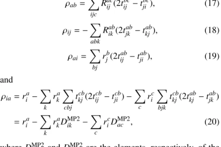
The required ˆR_µ2 intermediates, having different expressions for the two different kinds of spin multiplicity, are defined in step 4 of the algorithm in TableIand are obtained using the

R_µ2 =−X

ν1

A_µ2ν1r_ν1

ε_µ2−ω_ADC(2) (12)

amplitudes. The additional advantage of solving the rearranged pseudo-eigenvalue problem of Eq.(7) is that theR_µ2 ampli- tudes can be computed “on-the-fly” and their storage is not required.

Our implementation follows the ideas of H¨attig and Weigend presented for their density-fitting LR-CC2 algo-

rithm.¹⁹ The main difference is that our working equa- tions are written in the MO basis instead of the atomic orbital (AO) representation of Ref. 19 in order to effi- ciently utilize the reduced number of orbitals in the com- pressed NO basis. In the DF approach, the four-center two-electron integrals are approximated in a product form as

(pq|rs)=X

Q

J_pq^QJ_rs^Q, (13) where capital indices, such as Q, denote the functions of the auxiliary basis set and the J quantities are built from two- and three-center two-electron integrals, (P|Q) and (pq|P),

TABLE I. Algorithm and working equations for calculating the sigma vector for singlet and triplet excitations.

0. Perform MP2 calculation and store intermediateY_ai^Q=P

jbJ_jb^Q(2t^ab_ij −t_ji^ab) 1. Calculate intermediatesX^Q,X_ij^Q, andX^Q_ia

X^Q=2P

iaJ_ia^Qr_i^a X_ij^Q=P

aJ_ia^Qr_j^a X_ia^Q=P br_i^bJ_ba^Q 2. Add purelyr_i^a-dependent contributions toσiaand constructFia

if singlet:σia←P QJ_ia^QX^Q Fia=−P

jQJ_ja^QX^Q_ij +σia if triplet:Fia=P

jQJ_ja^QX_ij^Q σia← −P

jQJ_ij^QX_ja^Q+ (εa−εi)r_i^a

3. Compute ˆt_ij^ab, add corresponding contributions toσia (ia|jb)=P

QJ^Q_iaJ_jb^Q

if singlet: ˆt^ab_ij =[2(ia|jb)−(ja|ib)]/D^ab_ij] if triplet: ˆt^ab_ij =(ja|ib)/D^ab_ij

σia←¹₂P jbˆt_ij^abFjb if singlet:σia←¹₂P

jbP

kc[2(ia|jb)−(ja|ib)]r_k^cˆt_jk^bc if triplet:σia←¹₂P

jbP

kc(ja|ib)r_k^cˆt_jk^bc 4. Construct theJ^Q_ialist, build intermediate ˆR^ab_ij

J^Qia=X_ia^Q−P jJ_ij^Qr^a_j (ia|jb)=P

QJ^Q_iaJ_jb^Q (ia|jb)=P QJ^Q_iaJ^Q_jb

if singlet: ˆR^ab_ij =[2(ia|jb)−(ja|ib) + 2(ia|jb)−(ja|ib)]/(D_ij^ab+ωADC(2))

=(2R^ab_ij −R^ab_ji)/(D^ab_ij +ωADC(2))

if triplet: ˆR^ab_ij =[2(ia|jb)−(ja|ib)−(ja|ib)]/(D^ab_ij +ωADC(2)) Y^Q_ia=P

jbRˆ^ab_ijJ_jb^Q

5. Add the remaining contributions toσia σia←P

QbJ_ab^QY^Q_ib σia← −P

QjJ_ij^QY^Qja σia←¹₂P

jP

Qb(J_ib^QY_jb^Q+J_jb^QY_ib^Q)r_j^a σia← −¹₂P

bP

Qj(J_jb^QY_ja^Q+J_ja^QY_jb^Q)r_i^b

respectively, as

J_pq^Q =X

P

(pq|P)(P|Q)^−1/2. (14) The steps of the algorithm are given in detail in TableI.

Inspecting the algorithm, one finds the construction of inter- mediates ˆt_ij^ab and ˆR^ab_ij (steps 3 and 4) from the three-center integrals and the contraction of the latter with the J_jb^Q list (step 4) as the rate-determining steps of the iterative pro- cess. The operation count for these steps is proportional to n²_occn²

virtn_aux, wheren_occ(n_virt) denotes the number of occupied (virtual) orbitals and n_aux stands for the number of auxil- iary functions. Since the effective Jacobian, and thus σ as well, depends on the excitation energy, the non-linear eigen- value problem cannot be solved simultaneously for all excited states. To solve the eigenvalue equations effectively, a pro- cedure using a modified Davidson algorithm and the direct inversion in the iterative subspace (DIIS)⁸⁷ algorithm was implemented.^19,86

At the end of the iteration, the converged ADC(2) wave function is normalized, which is necessary for the evalua- tion of transition moments. To achieve this in spatial orbital basis, the amplitudes obtained are divided by the normalization

constant c=

s X

aibj

R^ab_ij R^ab_ij −1 2

X

aibj

R^ab_ij R^ab_ji +X

ai

r_i^ar_i^a. (15) Then the transition density matrix required for the ground to excited state transition moments can be obtained as

ρ_pq=hΨ^MP1|p⁺q⁻|Ψ^ADC(2)i

=h0|(1 +T₂^†)p⁺q⁻(R1+R₂)(1 +T₂)|0i

=h0|p⁺q⁻R₁|0i+h0|T₂^†p⁺q⁻R₁|0i

+h0|T₂^†p⁺q⁻R₁T₂|0i+h0|T₂^†p⁺q⁻R₂|0i. (16) This expression is often simplified^88,89 by discarding dis- connected contributions and by neglecting the higher than fifth-power scaling second-order terms. It can be shown that, analogous to LR-CC2, the resulting ADC(2) density matrix is consistent with the LR-CC theory and correct up to the first order. Our working equations for the transition density matrix in the spatial orbital basis are given for its various blocks by

ρ_ab=X

ijc

R^ac_ij(2t_ij^bc−t_ji^bc), (17) ρ_ij =−X

abk

R^ab_ik(2t_jk^ab−t_kj^ab), (18) ρ_ai =X

bj

r^b_j(2t_ij^ab−t_ji^ab), (19) and

ρ_ia=r_i^a−X

k

r_k^aX

cbj

t_kj^cb(2t^cb_ij −t^cb_ji)−X

c

r^c_i X

bjk

t_kj^cb(2t^ab_kj −t_jk^ab)

=r_i^a−X

k

r_k^aD^MP2_ik −X

c

r_i^cD^MP2_ac , (20) whereD^MP2_ik andD^MP2_ac are the elements, respectively, of the occupied-occupied and the virtual-virtual block of the MP2 one-particle density matrix, andR^ab_ij of Eq.(12)is, in practice, built from the intermediates of step 4 of TableIas

R^ab_ij =(ia|jb) + (ia|jb) D^ab_ij +ωADC(2)

. (21)

B. Construction of the reduced subspace

We have shown previously that, while preserving the intrinsic accuracy of the LR-CC2 excitation energies, the dimension of the virtual subspace can be significantly reduced by discarding NOs with low occupation numbers. On the other hand, the analogous frozen occupied NO approximation was found to be far less efficient for LR-CC2.⁸⁶We experienced similar trends in the case of ADC(2), therefore we restrict the present discussion to the application of frozen virtual NOs. If they are of interest, the working equations required for the frozen occupied NO approximation can be obtained analogously.

First, the virtual-virtual block of the one-particle density matrix is constructed from a lower-level wave functionΨ,

D_ab=hΨ|a⁺b⁻|Ψi. (22)

The eigenvectors of this matrix are the virtual natural orbitals (VNOs), while its eigenvalues are interpreted as the corre- sponding occupation numbers of the VNOs. If Ψ is appro- priately chosen, the NOs with smaller occupation numbers usually give a smaller contribution to the correlation or exci- tation energies. Therefore, in the frozen NO approximation, the NOs with occupation numbers below a predefined thresh- old, ε_VNO, are disregarded. The remaining VNOs will be denoted with a tilde (e.g., ˜a, ˜b,. . .), and the integral lists trans- formed to the VNO basis will also be distinguished with tildes (e.g., ˜J).

We have also demonstrated that the state-specific VNOs obtained from state-averaged density matrices are most suit- able to efficiently compute LR-CC2 singlet excitation ener- gies.⁸⁶The state-averaged density matrix we have introduced is defined as D = (D^MP2 + D^CIS(D))/2, where D^MP2 and D^CIS(D) denote the density matrices obtained from the MP1 and the configuration interaction singles with perturbative dou- bles [CIS(D)] wave functions. The one-particle MP2 density matrix in a spatial orbital basis can be expressed in the form of

D^MP2_ab =X

ijc

(2t_ij^cat_ij^cb−t^ca_ijt^bc_ij). (23) The CIS(D) density matrix,D^CIS(D), is obtained as the sum of the density matrices derived from the CIS wave function and its second-order perturbative correction (D),D^CIS(D) = D^CIS + D^(D). The CIS density matrix expressed in spatial orbitals reads as

D^CIS_ab =X

i

c^a_ic^b_i (24) for both the singlet and the triplet states, where c_i^a is a CIS coefficient. The spin adaptation results in different expressions for matrixD^(D)in the singlet and triplet cases. The expression for a singlet state is practically the same as for the MP2 density, Eq.(23), the only difference is that the MP2 amplitudes are substituted by the CIS(D) doubles coefficients. The latter can be expressed as

c^ab_ij =

Pc[(ac|bj)c^c_i + (ai|bc)c^c_j]−P

k[(kj|ai)c^b_k+ (ki|bj)c_k^a]

D_ij^ab+ω_CIS ,

(25) whereω_CIS stands for the CIS excitation energy.^90,91 For an excited state of triplet multiplicity, the virtual-virtual block of matrixD^(D)is given as

D^(D)_ab =X

ijc

(c^ca_ijc^cb_ij +c^ca_ijc^cb_ij −c^ca_ijc^bc_ij), (26) where the c^ab_ij coefficients are still defined by Eq.(25), but they are built using the triplet CIS coefficients and excitation energy. Furthermore,c^ab_ij denotes the triplet-coupled CIS(D) doubles coefficient, which is evaluated as

c^ab_ij =

Pc[(ac|bj)c^c_i −(ai|bc)c^c_j] +P

k[(kj|ai)c_k^b−(ki|bj)c^a_k]

D_ij^ab+ω_CIS .

(27) The algorithms and the working equations for the computa- tion of the singlet density matrix were published previously.⁸⁶ The analogous steps and expressions for the triplet case are

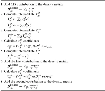
TABLE II. Working equations for the evaluation of the triplet CIS(D) density matrix.

1. Add CIS contribution to the density matrix D^CIS(D)_ab ←P

ic_i^ac^b_i 2. Compute intermediateY_ai^Q

Y_ai^Q←P cJac^Qc^c_i Y_ai^Q← −P

jJ_ij^Qc^a_j 3. Compute intermediateV_ij^ab

V_ij^ab=P QY_ai^QJ_bj^Q 4. Calculatec^ab_ij coefficients

c_ij^ab=(V_ij^ab+V_ji^ba)/(D^ab_ij +ωCIS) 5. Compute intermediateX_ij^ab

X_ij^ab=c^ab_ij −c^ba_ij

6. Add the first contribution to the density matrix D^CIS(D)_ab ←P

ijcc^ca_ijX_ij^cb 7. Calculatec^ab_ij coefficients

c^ab_ij =(V_ij^ab−V_ji^ba)/(D^ab_ij +ωCIS)

8. Add the second contribution to the density matrix D^CIS(D)_ab ←P

ijcc^ca_ijc^cb_ij

given in detail in TableII. Note that the one-particle MP2 den- sity matrix is only constructed once, for the ground state. On the contrary, the CIS(D) wave function and hence the CIS(D) density matrix have to be evaluated for each excited state.

The rate-determining step of the density matrix calculation, for both MP2 and CIS(D), is the assembly of the four-index integral list of intermediateV(step 3), which is a fifth-power scaling operation with costs proportional ton²_occn²

virtn_aux. The algorithm contains two additional fifth-power scaling opera- tions (steps 6 and 8) with computational expenses proportional ton²_occn³

virt, while there is only one such term in the case of MP2 or singlet CIS(D).

In our previous LR-CC2 study, we have also introduced a simplification to the MP2 and (D) density matrices, with which the NO approximation works similarly well. Here we again take advantage of the neglect of the exchange-like terms from the corresponding density matrix expressions.

With that approximation Eqs.(23)and(26)read, respectively, as

D^MP2_ab =X

ijc

2t^ca_ij t^cb_ij (28) and

D^(D)_ab =X

ijc

(c^ca_ijc^cb_ij +c^ca_ijc^cb_ij). (29) One benefit of this simplification is that the evaluation of intermediateX^ab

ij (step 5) can be omitted. In addition, the cor- responding contribution to the density matrix can be obtained more efficiently via the multiplication of the CIS(D) doubles coefficient matrix with its transpose (step 6). On top of that, the implementation of the algorithm becomes significantly easier even if the entire integral lists or intermediates cannot be kept in the memory.

As expected, the VNOs constructed as described above are only ideal for ADC(2) calculations if CIS(D) is a good approx- imation to ADC(2). The prerequisite for this is that the CIS method provides a qualitatively good description of the excited state. If the coefficients of double excitations are not stored, a

good measure for the quality of the CIS and CIS(D) approxi- mations is the overlap of the CIS and the single excitation part of the final ADC(2) wave functions. Our numerical experience shows that, if this overlap is relatively small, the ADC(2) calcu- lations performed in the reduced VNO space may yield inad- equate excitation energies and transition moments. In these cases, we found that the dominant excitations of the ADC(2) wave function obtained in the reduced space correspond to those of the CIS wave function, and particular excitations that have considerable weight in the canonical ADC(2) are miss- ing. This problem cannot be resolved by tightening theε_VNO threshold as the occupancy of the VNOs which do not notice- ably contribute to the CIS wave function is rather low. To overcome this problem, we found the following approach to be useful.

In practice, for a particular excited state, the orbital ener- gies of the canonical virtual orbitals contributing to the wave function are relatively close to each other. Thus, we can sup- pose that all the important orbitals will be included in the reduced space if it is augmented with the canonical virtual orbitals which are close in energy to the virtuals significantly contributing to the CIS wave function. For the selection of such orbitals, two further thresholds were introduced. First, those canonical virtual orbitals are chosen for which at least one CIS coefficient of an excitation involving them is greater than thresholdε_CIS. Second, all those canonical virtual orbitals are selected whose orbital energy is in a given interval. The lower limit of the interval is the orbital energy of the lowest MO selected in the first step minus threshold ε_E, while its upper limit is the orbital energy of the highest chosen MO plusε_E. The orbitals of the reduced VNO space are projected out of the selected canonical virtual orbitals, and the remaining orbitals are orthonormalized employing canonical orthogonal- ization dropping the eigenvectors of the overlap matrix with eigenvalues lower than 10⁷. The resulting orthonormal MOs are added to the reduced VNO space, and the orbitals of the extended space are canonicalized. In practice, it means that the Fock-matrix is transformed to the extended MO space, and the matrix is diagonalized. The resulting pseudo-canonical orbitals and the corresponding orbital energies will be used in the subsequent calculations. For the sake of simplicity, from now on, this pseudo-canonical basis will be referred to as the VNO basis.

So far an accurate lower-rank approximation to the MP2 and ADC(2) wave functions has been introduced by defining the corresponding state-specific VNO basis. Analogously, the auxiliary basis can also be compressed by finding an appro- priate basis transformation. It can be shown that the truncated singular vector basis of J gives the most efficient approxi- mation toJitself and hence to the corresponding assembled four-center integrals.⁸⁵ In practice, it is more economical to obtain the singular vectors as the eigenvalues of matrix W with elements

W_PQ=X

pq

J_pq^PJ_pq^Q. (30) Similar to the NO approach, the eigenvectors, the so-called NAFs, with eigenvalues below a predefined threshold,ε_NAF, are discarded in the compressed representation of J.

In the following, we will employ two different sets of NAFs. First, as in our previous LR-CC2 study, we construct NAFs to compress the representation of the integrals in the NO basis. Here we buildWof Eq.(30)using ˜J, the integral list transformed to the VNO basis. These NAFs will be referred to as restricted NO space NAFs or RS-NAFs for short. The RS-NAFs are suitable to reduce, for instance, the cost of cer- tain assembly andσ-vector construction steps of the ADC(2) calculation (see, e.g., Table I). Another option is to utilize the NAF approximation right at the beginning, as soon as the three-center integrals are transformed to the canonical HF MO basis. These NAFs will be called the complete MO space NAFs, or shortly, CS-NAFs, and the correspondingJintegrals will be denoted hereafter by ˆJ. We note here that, naturally, the CS-NAF basis is usually significantly larger than the RS- NAF basis but still represents a compressed, system-specific auxiliary basis with which the expenses of the CIS calcula- tion and density matrix evaluation steps can be cut roughly in half.

C. General algorithm

In this section, we briefly collect all the steps required for our reduced-cost ADC(2) algorithm. We introduce here two branches for test purposes in order to assess the accu- racy of the CS-NAF approximation, which was not present in our previous study.⁸⁶Algorithm 1 is basically the generaliza- tion of our VNO and (RS-)NAF approximation-based LR-CC2 scheme apart from the step that the VNOs selected using the ε_VNOthreshold are supplemented with the close-lying canoni- cal orbitals. This is extended in Algorithm 2 by the introduction of CS-NAFs as well (see step 2 below). Our general algorithm is as follows.

0. Solve HF equations

1. Construct the canonical integral listJ

2. If Algorithm 2: Calculate matrixWusing three-center integral listJ [Eq. (30)], and transform the auxiliary index ofJto the CS-NAF basis to obtain ˆJ

3. Solve CIS equations for all the excited states simultaneously using either J (Algorithm 1) or ˆJ (Algorithm 2)

4. Loop over excited states

4.a. Calculate the state-averaged one-particle density matrixD(TableII) using eitherJ(Algorithm 1) or ˆJ (Algorithm 2), and construct the truncated virtual space. Transform the MO indices ofJor Jˆto the VNO basis to obtain ˜J.

4.b. Calculate matrixWusing three-index integrals ˜J [Eq.(30)], and transform the auxiliary index of ˜J to the RS-NAF basis (J). Write integral listJto disk.

End loop

5. Loop over excited states

5.a. Retrieve integral listJfrom disk

5.b. Perform MP2 calculation and solve ADC(2) equa- tions (TableI)

End loop

We would like to point out that the CS-NAF approxi- mation affects the accuracy of all the quantities computed

subsequently, such as density matrices, VNOs, and RS-NAFs.

Besides that it is not guaranteed that the truncated RS-NAF basis of Algorithm 1 is a subset of the truncated CS-NAF basis even if the VNOs of the two algorithms can be con- sidered the same in the case of a highly accurate CS-NAF approximation. In other words, if both NAF approximations are employed, contributions to the retained RS-NAFs coming from the dropped CS-NAFs are present in Algorithm 1, but they are lost in Algorithm 2. Both of these error sources will be extensively investigated in Sec.III.

III. RESULTS

A. Computational details

The presented reduced-cost ADC(2) algorithm has been implemented in the Mrccsuite of quantum chemical programs and is available in the current release of the package.⁹²

For the benchmark calculations, Dunning’s correlation consistent basis sets augmented with diffuse functions (aug-cc- pVXZ, whereX= D, T, Q) were used,^93–95and the correspond- ing auxiliary bases developed by Weigendet al.were employed in both the HF and the excited-state calculations.^96–98 In the CIS and ADC(2) calculations, the core MOs were kept frozen.

To quantify the errors originating from our approxima- tions, a test set of small molecules was employed containing examples for all important types of excitation.⁸⁶Valence exci- tations (n → π^∗,π → π^∗, andσ → π^∗) are present among the transitions taken from the benchmark set of Thiel and co-workers.^99,100 We have also added a couple of the Ryd- berg excited states of these systems to our test set as well as the CT excitations of an ethylene-tetrafluoroethylene system

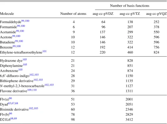
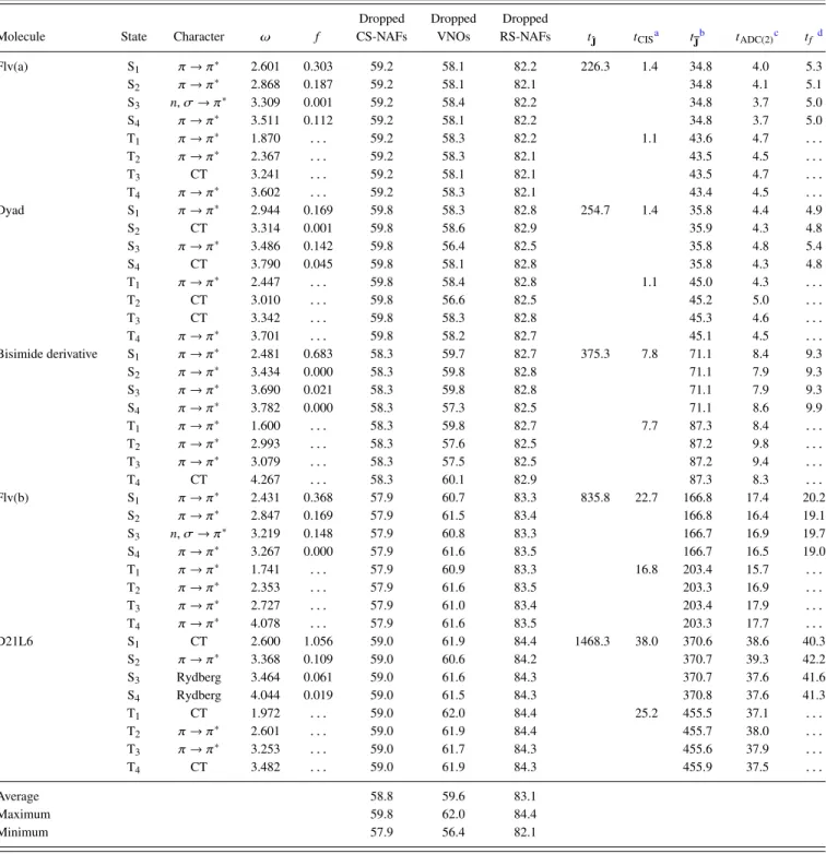
(10 Å separation, taken from the work of Dreuwet al.¹⁰¹). We have also assessed the accuracy of our approach on a more realistic set of systems containing seven medium-sized, fre- quently studied molecules.^86,102–110 Additional calculations were performed for even larger systems to demonstrate the efficiency of our implementation. For this purpose, molecules were taken from the studies of Grimme¹⁰³ and Sch¨utz and co-workers.^65–69 The systems included in the three sets are collected in TableIII, while their structures are shown in the supplementary material.

The reported computation times are wall-clock times determined on a machine equipped with 128 GB of main memory and a 6-core 3.5 GHz Intel Xeon E5-1650 processor.

B. Small molecules

First, we study the accuracy of our approximations on the example of the test set containing the smaller molecules.

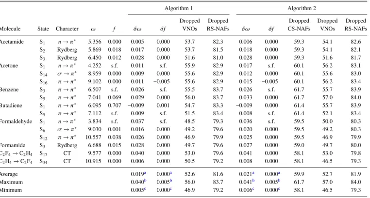
We analyze the accuracy of the singlet and triplet excitation energies as well as of the oscillator strengths correspond- ing to singlet transitions using the aug-cc-pVTZ basis set, which is probably the most relevant from the practical point of view; double- and quadruple-ζ-quality basis sets will be considered later. In order to find reliable default values for the VNO and NAF truncation thresholds, we rely on the results of our extensive convergence tests for εVNO and εNAF that we obtained for our related reduced-cost LR-CC2 scheme.⁸⁶ We found, with the default values ofε_VNO= 7.5×10⁵ and ε_NAF = 0.1 a.u., the mean absolute error (MAE) of the sin- glet LR-CC2 excitation energies to be about 0.02 eV, which is an order of magnitude smaller than the intrinsic error of LR-CC2.^111,112Considering the close relation of the formula- tion of ADC(2) and LR-CC2,¹¹³ their comparable numerical

TABLE III. The size of the systems studied and the number of the basis functions in the basis sets considered.

Number of basis functions

Molecule Number of atoms aug-cc-pVDZ aug-cc-pVTZ aug-cc-pVQZ

Formaldehyde^99,100 4 64 138 252

Formamide^99,100 6 96 207 378

Acetamide^99,100 9 137 299 550

Acetone^99,100 10 146 322 596

Butadiene^99,100 10 146 322 596

Benzene^99,100 12 192 414 756

Ethylene-tetrafluoroethylene¹⁰¹ 12 220 460 824

Hydrazone dye¹⁰⁵ 21 828

Diphenylamine¹⁰⁵ 21 851

Azobenzene¹⁰⁵ 24 874

6,6⁰-difluoro-indigo^102,103 28 1150

Bithiophene derivative^102,103 29 1135

N-methyl-2,3-benzocarbazole^102,103 31 1127

Flavone derivative^109,110 36 1311

Flv(a)⁶⁶ 51 2001

Dyad^65,67,68 53 2051

Bisimide derivative^102,103 60 2346

Flv(b)⁶⁶ 78 2829

D21L6^68,69 98 3412