Equilibrium solubility measurement of ionizable drugs – consensus recommendations for improving data quality

Open Access : ISSN : 1848-7718

http://www.pub.iapchem.org/ojs/index.php/admet/index White paper

Equilibrium solubility measurement of ionizable drugs – consensus recommendations for improving data quality

Alex Avdeef,

Elisabet Fuguet,

Antonio Llinàs,

Clara Ràfols,

Elisabeth Bosch,

Gergely Völgyi,

Tatjana Verbić,

Elena Boldyreva

, Krisztina Takács-Novák

1 in-ADME Research, 1732 First Avenue, #102, New York, NY 10128, USA

2 Departament de Química Analítica and Institut de Biomedicina (IBUB), Universitat de Barcelona, Martí i Franquès 1-11, E- 08028 Barcelona, Spain

3 Serra-Húnter Program, Generalitat de Catalunya, Barcelona, Spain

4 RIA iMED DMPK, AstraZeneca R&D, Gothenburg, Sweden

5 Semmelweis University, Dept. of Pharmaceutical Chemistry, H-1092 Budapest, Högyes E. u.9, Hungary

6 Faculty of Chemistry, University of Belgrade, Dept. of Analytical Chemistry, Studentski trg 12-16, Belgrade 11158, Serbia

7 Institute of Solid State Chemistry and Mechanochemistry SB RAS, Kutateladze, 18, Novosibirsk, 630128 Russia

*Corresponding Author: E-mail: Alex@in-ADME.com; Tel.: +1-646-678-5713 Received: May 08, 2016; Revised: June 21, 2016; Published: June 29, 2016

Abstract

This commentary addresses data quality in equilibrium solubility measurement in aqueous solution. Broadly discussed is the “gold standard” shake-flask (SF) method used to measure equilibrium solubility of ionizable drug-like molecules as a function of pH. Many factors affecting the quality of the measurement are recognized.

Case studies illustrating the analysis of both solution and solid state aspects of solubility measurement are presented. Coverage includes drug aggregation in solution (sub-micellar, micellar, complexation), use of mass spectrometry to assess aggregation in saturated solutions, solid state characterization (salts, polymorphs, cocrystals, polymorph creation by potentiometric method), solubility type (water, buffer, intrinsic), temperature, ionic strength, pH measurement, buffer issues, critical knowledge of the pKa, equilibration time (stirring and sedimentation), separating solid from saturated solution, solution handling and adsorption to untreated surfaces, solubility units, and tabulation/graphic presentation of reported data. The goal is to present cohesive recommendations that could lead to better assay design, to result in improved quality of measurements, and to impart a deeper understanding of the underlying solution chemistry in suspensions of drug solids.

Keywords

shake-flask solubility; intrinsic solubility; water solubility; buffer solubility; thermodynamic solubility; Bjerrum curve; CheqSol; Potentiometric Cycling for Polymorph Creation; Henderson-Hasselbalch equation; aggregates;

oligomers; micelles; hydrates; salts; polymorphs; cocrystals.

Introduction

Many investigational compounds in pharmaceutical development are practically insoluble solids consisting

of ionizable molecules. Interpreting their solution properties in the course of measuring solubility – as a function of pH – can be problematic. Although there are a multitude of published methods, today’s druglike molecules can pose special challenges, perhaps not adequately addressed in practice. The published literature is replete with incomplete/ambiguous and potentially misleading examples of solubility reports, frequently documented inconsistently. The solubility methodology appears to be in need of a timely tune up.

This commentary discusses ways to improve the measurement of thermodynamic solubility of druglike substances in aqueous media. (Topics such as solubility in bio-relevant media, kinetic solubility, and solubility of amorphous and of liquid-liquid phase separated (LLPS) solids are outside of its scope.) It is relatively scarce to find many high-quality solubility measurements that adequately cover the chemical space of drugs and research compounds. Measuring such data is expensive and analytical-resource consuming. Even with great expense, quality is not ensured when results are determined from under-designed assays. The “Solubility Challenge” from Llinàs et al. [1] and Hopfinger et al. [2] has spurred fresh discussion about data quality in solubility measurement in pharmaceutical research. Concomitantly, Baka et al. [3] examined the classical saturation shake-flask method, to assess which experimental conditions significantly affect the measured equilibrium solubility. More recently, solubility data quality has been reviewed by Avdeef [4].

Optimal experimental design to measure the aqueous equilibrium solubility of an ionizable substance requires a number of critical considerations. Briefly, the aqueous medium to which the substance is added ideally contains a buffer to help control the pH. To this medium, the substance may be added in a number of ways: (a) as a highly supersaturated aqueous solution, (b) as a saturated hot solution, (c) as a concentrated solution in a water-miscible organic solvent, or (d) as a solid – which may or may not be in a thermodynamically stable form. The first three approaches are precipitation routes, while the fourth involves dissolution. The latter process is most commonly used, best understood, and is the backbone of the commentary here.

Solubility reactions, being heterogeneous, are often slow to reach equilibrium, especially in the case of low- soluble substances. With sufficient added solid and enough time, chemical equilibrium is expected, where the substance in its stable crystalline form is in dynamic equilibrium with its solution form. As the dissolution proceeds, the solid phase can re-precipitate as another form with another structure (polymorphic transitions) and even another composition (formation of crystal solvates, salts, or loss of solvate from the starting solid).

Dissolution of multi-component solids (salts – formed by cations and anions, or cocrystals – formed by neutral molecules, a drug and another molecule, termed a “coformer”, which are often strongly hydrogen-bonded) adds complexity, since on their dissolution, re-crystallization of some components can start, depending on the solution conditions. The values of the solubility measured at different time points will therefore correspond to different solid phases, not necessarily the one initially introduced into solution. Sometimes a long equilibration time is needed to settle to the most stable crystalline form. In solution, the substance may undergo ionization, self-aggregation (forming water-soluble dimers, trimers, etc., or micelles in the case of amphiphilic substances), or complexation with some of the buffer components. In some cases, solids dissolve as clusters of molecules, which can be preserved for some time before being broken apart by the solvent. At true dynamic equilibrium, the forward (dissolution) and reverse (precipitation) reaction rates are equal to one another. In this dynamically equilibrated saturated solution, the concentration of the drug substance (summed over all of its dissolved forms) is the solubility. Both phases of the solubility process are important to consider, as

measured solubility depends both on the solid and the solution forms. Since the solubility is temperature dependent, the temperature needs to be controlled. For ionizable substances, solubility depends on pH, so the final (equilibrium) pH of the saturated solution, pHsat, needs to be measured directly.

Methods of characterizing the solid state (powder X-ray diffraction, differential scanning calorimetry, FT-IR reflectance/Raman spectra of slurries, elemental analysis, etc.) are well established. This is an important consideration with actionable consequences, since patents may be issued to cover particular solid state forms of a marketed drug substance.

However, characterizations of the solution state of ionizable substances of sparingly-soluble or amphiphilic substances that are surface active are far less well explored. This is especially true of ionizable substances in saturated solutions above their critical micelle concentration (CMC), with the assay temperature being above the Krafft point [5]. Under such circumstances, crystalline solids of the substance are effectively in equilibrium with micelles (or sub-micellar aggregates), in some cases leading to the transient formation of oils if the melting point of the neutral form of the substance is not far above the assay temperature. Such solutions can be very sensitive to changes in pH and/or temperature, as well as by the presence of background salts and other excipients [6].

This commentary is the outgrowth of discussions held during the “Thermodynamic Solubility Measurement of Practically Insoluble Ionizable Drugs – Case Studies & Suggested Method Improvements” session at the 4^th World Conference on Physico Chemical Methods in Drug Discovery and Development (PCMDDD-4, http://www.iapchem.org/page.php?page_id=56), held on Red Island, Croatia, 21-24 September 2015. The session focused on discussing the best practices for the saturation shake-flask measurement of solubility as a function of pH (the “gold standard” methodology), along with promising potentiometric methods, and attempted to reach a consensus about the best approaches for studying sparingly soluble drug substances. A questionnaire was prepared and distributed to the attendees. The responses received from several of the participants are summarized in Appendix D.

Several excellent books and reviews serve as background material for the commentary covering the solubility of druglike molecules: general coverage of solubility [7-10]; salt formation/selection [11-16];

polymorphism [17-20]; analysis of saturated solution speciation [21-27]; dissolution/solubility of cocrystals [28-37]; anhydrous forms versus hydrates [16, 38, 39].

Case Studies

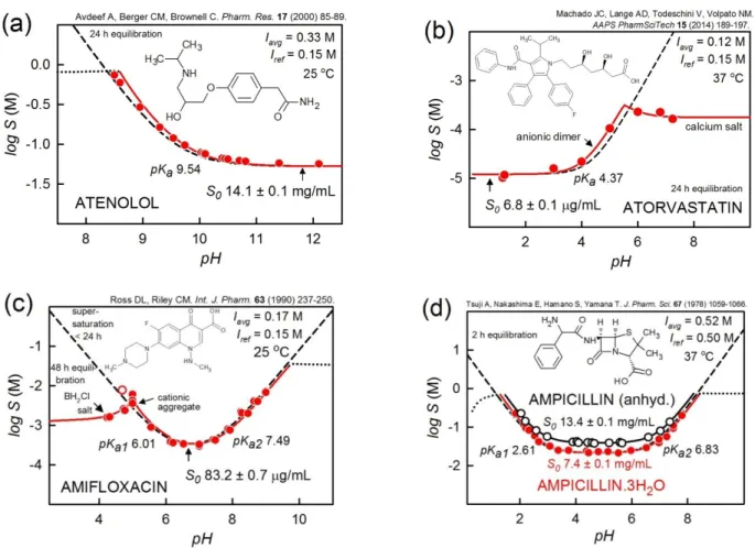
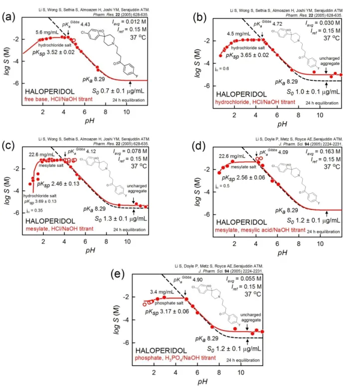
The commentary begins with several selected case studies of molecules which illustrate appreciable challenges encountered in the measurement of solubility. Figure 1 shows four examples of drugs which reveal relatively simple logS-pH profiles, which can be more or less predicted by the Henderson-Hasselbalch (HH) equation [27, 40, 41]. Figure 2 shows three examples of molecules with logS-pH profiles that are consistent with the presence of anionic or uncharged self-associated aggregates, and one case consistent with drug- buffer interaction. Figure 3 illustrates the logS-pH profiles of haloperidol resulting from different salt precipitations, illustrating some degree of supersaturation for two cases near the Gibbs pKa [42, 43] in the pH 4.1-4.9 interval and the possible formation of uncharged aggregates for pH>8. Figures 4 and 5 ratchet up the complexity of logS-pH profiles of surface-active molecules which precipitate both as salts and as uncharged species.

The examples were selected to show that care needs to be exercised in interpreting the shapes of the solubility-pH

profiles [21-25] and that assays need to be optimized to enhance the confidence in the interpretations of the data.

Figure 1. Four examples of drugs which reveal relatively simple logS-pH profiles, which can be more or less predicted by the Henderson-Hasselbalch equation.

The following logS-pH curve notations are used (except Figures 4b and 5b):

 The dashed curves refer to the profiles calculated from the simple HH equation (not corrected for ionic strength or dilution effects)

 The solid curves are calculated using the refined constants from fitting the measured logS-pH data (filled circles) to the proposed equilibrium model, using the pDISOL-X program (in-ADME Research;

www.in-adme.com/pdisol_x.html)

 The dotted curves indicate regions of pH of subsaturation, where the substances are dissolved

 S0 refers to the intrinsic solubility of the uncharged form of the substance

 pKsp refers to the negative log of the salt (or cocrystal, as in later sections) solubility product

 The reference and average ionic strengths are indicated as Iref and Iavg, respectively. The former values correspond to the pKa determination conditions. Corrections are made for changes in the ionic strength in the solubility assays, as described by Völgyi et al. [22] and Wang et al. [44]

 The jH coefficients (Figure 3b,c,d) refer to estimated pH electrode junction potential factors [45] in very acidic solutions (pH < 1), as detailed in Appendix C.

Atenolol

Figure 1a shows the logS-pH profile of atenolol [46]. Since the weak base is relatively soluble, it takes a 3.8 M atenolol solution (1 g of the free base added to 1 mL of 50 mM phosphate buffer) to span the concentration range shown in the figure. The ionic strength rises from 0.24 to 0.83 M as pH is lowered from 9.5 to 8.5 using 1 M HCl. Such pH adjustment is accompanied by a very large dilution effect. This requires that the pH electrode used be well-calibrated. Since the accurate pKa of atenolol is known, the fit can be further improved over what is shown, by assuming the presence of a neutral aggregate species, (Case 1b in [27]); the standard deviation drops from 0.047 to 0.015 log unit. The intrinsic solubility is slightly lessened from 14.1 to 11.0 mg/mL. The performance of the pH electrode is quite important in this case study.

Atorvastatin

Figure 1b shows the logS-pH profile of atorvastatin added as the calcium salt [47]. This example illustrates the need to know the pKa accurately. The value of 4.37 at 37 ^oC was predicted [26] from the measured value at 25 ^oC [48]. If 4.37 is the correct value, then the small parallel displacement of the solubility values in the pH 4-5 region to lower pH is consistent with the presence of half-ionized aggregates, [AH.A^–]n, (Case 3a in [27]). On the other hand, it could be assumed that the reported pKa is inaccurate, and that no aggregates form in the pH 4-5 region. Then, the ionization constant determined by pDISOL-X would be 3.94 ± 0.09, using the logS-pH data, based on methods popularized in older literature [49, 50]. Such a big difference (0.43 log unit) seems unrealistic, so the case for aggregation cannot be easily dismissed.

For the aggregate model in the figure, as the pH is increased from 1 to 5, the only solid present in the suspension is the free acid, HA. As pH increases to 5, the free [Ca²⁺] remains constant at 1.78 mM, as [A^–] increases. When pH 5 is reached, the salt solubility product is exceeded and the calcium salt of the drug, CaA2(s), begins to co-precipitate with HA(s) until pH 5.5. Between pH 5.0 and 5.5, the calcium concentration decreases by the same extent as that of atorvastatin anion increases, but the product [Ca²⁺][A^–]2 remains constant. This is the pH interval containing two different solids. Above pH 5.5 (the point of maximum solubility), all HA(s) dissolves, as [Ca²⁺] levels off at 0.09 mM, and only the calcium salt is predicted to precipitate, as the above product of concentrations remains constant. It may be surprising that as an added calcium salt, atorvastatin does not have a distinct Gibbs pKa [42, 43], but rather shows co-precipitation over a 0.5 pH interval. Had the precipitate been between the drug and sodium ions, there would have been a distinct pKaGibbs

. The system is complex and several models can be proposed to rationalize the logS-pH profile. As can be seen, the independently-determined pKa is critical to the analysis of the data. It would have been important to isolate and characterize the solids, at least by elemental analysis, if not by comparison to PXRD of demonstrated crystalline solids of known stoichiometry. Sufficiently sensitive computations tools are needed to fully interpret such complicated systems.

Amifloxacin

Figure 1c shows the logS-pH profile of amifloxacin, an ampholyte which forms a hydrochloride salt below pH 5 [51]. The region of maximum solubility near pH 5 showed supersaturation effects, especially at equilibration times < 24 h. The data in the figure are based on 48 h equilibration time. The unfilled circle was assigned zero weight in the refinement, since no equilibrium model could be found to fold the point into the curve represented by the other points. Also, the region between pH 5 and 6 indicated the presence of a small

amount of Case 2b-type in [27] cationic dimeric aggregate. This example illustrates the time dependence of the measured solubility.

Ampicillin and Ampicillin Trihydrate

Figure 1d shows the logS-pH profiles of two forms of ampicillin: anhydrous (unfilled circles) and trihydrate (filled circles) [52]. It is noteworthy that the equilibration times were 2 h in both cases. Had longer dissolution times been used, the more soluble anhydrous form would likely have converted into the trihydrate. Many anhydrous forms of drugs are near 2-fold higher in solubility than their hydrate counter parts [4, 18]. The two profiles are well-described by the simple HH equation.

Cefadroxil

Figure 2a shows the logS-pH profile of cefadroxil, which illustrates two complicating aspect of solubility equilibria [53]. The study considered many different buffers: acetate, ammonium, borate, citrate, formate, lactate, and phosphate. The analysis of the data here excluded the measurements in citrate (unfilled squares)

Figure 2. Shown are three examples of molecules with logS-pH profiles which are consistent with the presence of anionic or uncharged self-associated aggregates, and one case consistent with drug-buffer interaction.

and lactate (unfilled circles) buffers, since their solubility in acidic solutions tended to deviate from the curve composed of all the other buffer measurements. The elevated solubility of the lactate and citrate cases suggested that complexes might have formed between the buffer anions and the positively-charged cefadroxil, complicating the solution chemistry. The analysis of the non-complicating buffer data yielded the solid curve in the figure. Evidently, the data above pH 6 cannot be predicted by the simple HH equation. Using pDISOL-X, the

data were best fit by assuming the presence of anionic monomers and trimers (Case 2a in [27]) of cefadroxil.

Shoghi et al. [53] proceeded to analyze the solutions between pH 6 and 7 using low ionization energy ESI-Q- TOF-MS/MS and found direct evidence for the presence of monomers, dimers and trimers in saturated solution. This example illustrates the importance of corroborating proposed solution-phase equilibrium models by independent methods.

Diprenorphine

Figure 2b shows the solubility profile of diprenorphine hydrochloride, XH2.Cl, in the modified Sørensen’s buffer: 0.15 M NaH2PO4 adjusted with 14.85 M H3PO4 or 0.5 M NaOH [22]. The two pK^a values of diprenorphine were carefully determined in the study by Völgyi et al. [22]. For pH>pKaGibbs

5.07, the precipitate is the uncharged ordinary ampholyte, showing the characteristic parabolic shape. At pH below the Gibbs pK^a, either the chloride or the phosphate salt precipitates (or possibly both). Based on the reported solubility data, it is not definitively certain which form precipitates. More data would be needed at very low pH. Alternatively, the salts could have been isolated and characterized. The flat shape of the curve pH 2-5 is most consistent with chloride precipitate. A phosphate precipitate would be expected to show an upward curvature near the pK^aGibbs. At pH>9, the logS-pH curve shows a shift to lower pH, compared that what would be predicted from the simple HH equation. The consistent interpretation of the shift is that a water-soluble mixed-charge anionic dimer forms, with the basic stoichiometry XHX^–(Case 3a in [27]).

Ametryne

Figure 2c shows the solubility profile of ametryne [54], a weak base that appears to show free-base aggregation (Case 1b in [27]). As reported, there was no indication of supersaturation effects at the 24 h equilibration. The pKa was spectrophotometrically determined [55]. Several other derivatives (but not all) studied by Ward and Weber [54] showed the characteristic Case 1b logS-pH pattern. If the free-base aggregation model were not invoked, then the refined pKa would be 3.14 ± 0.08, almost a log unit lower than the measured value. This example illustrates the need for independently measuring the pKa, under conditions free of effects of aggregation and precipitation. Also, a mass spectrophotometric analysis of the slurry in neutral solution would have been corroboratively valuable.

Haloperidol

The salt solubility of haloperidol described by Li et al. [56, 57] raises several interesting points in assay design and data interpretation. Figure 3 illustrates the pH-dependent formation of three crystalline salts of haloperidol: hydrochloride, mesylate, and phosphate.

In the first three frames of the figure, HCl or NaOH were used to adjust the pH of haloperidol, either introduced as a free base (Figure 3a) or as a hydrochloride (Figure 3b). Within the bounds of experimental errors, the results are largely the same. The data in the hydrochloride case (Figure 3b) above pH 8 indicate a non-HH effect, which can be due to three situations: (i) formation of uncharged aggregates (Case 1b in [27]), or (ii) 24 h time not being adequate to reach full equilibration, or (iii) the formation of an oil phase (liquid-liquid phase separation, LLPS [58, 59]), which is more soluble than the free-base crystalline phase (melting point, 149 °C). Ignoring this [49, 50], the logS-pH data above pH 7 might suggest that the pKa of haloperidol at 37 °C is 8.0. This would not be in agreement with the pKa 8.29 independently determined at 37 °C [60] and 8.60 at

25 °C [61]. Based solely on the solubility measurements, none of the three possibilities can be definitively ruled out, and additional investigation might be desirable.

Figure 3. Examples of logS-pH profiles of haloperidol resulting from different salt precipitations, illustrating some degree of supersaturation near the Gibbs pKa in the pH 4.1-4.9 interval and the possible formation of uncharged

aggregates for pH>8 (see text).

Figure 3c depicts the titration of the haloperidol mesylate salt by either HCl or NaOH. The higher solubility in the salt precipitation region (pH 2-4) compared to that in Figures 3a and 3b suggests that the precipitate is the mesylate salt of haloperidol. However, the five lowest-pH points (Figure 3c) are not indicative of a mesylate salt. At the lowest pH, the data were better fitted with the Ksp corresponding to the hydrochloride

salt. Because of the very low pH (<1), it was necessary to invoke a pH electrode junction potential effect (jH=+0.35 [45]; cf., Appendix C). This was also needed in the cases of Figure 3b and 3d, for pH  1. In the low-pH mesylate example, there is actually a region predicted to contain co-precipitates of both BH.Cl(s) and BH.mesylate(s). Figure 3d is an example of haloperidol introduced as the mesylate salt and titrated with either mesylic acid or NaOH. The same solubility is evident in the pH 2-4 region as that shown in Figure 3c. The precipitous drop in solubility at low pH in Figure 3c arises as a “common ion” effect, namely that in the pH 2-4 region, the concentration of chloride contributed by the HCl titrant is not high enough to exceed the solubility product of BH.Cl(s), until enough HCl had been added to reach the very low pH values (pH<2).

In Figures 3c and 3d, the unfilled circles were assigned zero weights in the regression analysis. The reasonable explanation for their deviancy from the models is due to supersaturation effects.

Figure 3e is an example of haloperidol introduced as the phosphate salt and titrated with either phosphoric acid or NaOH. No way was found to rationalize the three points (unfilled circles) with the lowest pH, so they were assigned zero weights.

It is interesting to note in the haloperidol case study that the order of drug salt solubility (pH 2-4) is:

mesylate (23 mg/mL) > chloride (5 mg/mL) > phosphate (3 mg/mL). However, the order of the negative log salt solubility products is different: mesylate (2.5) < phosphate (3.2) < chloride (3.5). This highlights the notion that salt solubility is a conditional constant, depending on the concentrations of both the drug and the counterion, whereas the salt solubility product is a true equilibrium constant.

As is evident, the interesting haloperidol case study invokes several issues where experimental design has significant consequences: titrant used to adjust pH, electrode calibration, supersaturation, and possibly aggregation (or related phenomena).

Thiazolyloxamic Acid Derivative

Figure 4 shows a very complex solubility-pH profile of a surface-active weak acid, N-[4-(1,4-benzodioxan-6- yl)-2-thiazolyl]oxamic acid, which has two pKas: 1.32 and 10.31, both determined spectrophotometrically [6]. It is an example of a molecule, when added as a salt, that becomes more soluble as more of it is added to solution, somewhat like the case of amiodarone [24]. The prominent “bump” in the logS-pH profile is consistent with the formation of a hexameric anionic aggregate, (HA^–)6. The solubility of the ethanolamine salt in the neutral pH region is 20.3 mg/mL (pKsp 4.22). Since aggregation is strongly dependent on concentration, in the absence of aggregation (i.e., at lower concentrations), the salt solubility would be predicted to be 2.0 mg/mL (simulated blue curve in Figure 4a). Here, salt solubility depends not only on the amount of ethanolamine but also the amount of the conjugate anion, which in turn is affected by the extent of aggregation. Pandit et al. [6] also studied other salt-forming counterions, besides ethanolamine. Figure 4a shows the calcium salt solubility (dash-dot curve). The calcium salt is quite a bit less soluble than the one based on ethanolamine. For the case of calcium, the impact of aggregation is much lessened, as is suggested in Figure 4a.

Figure 4. N-[4-(1,4-benzodioxan-6-yl)-2-thiazolyl]oxamic acid as an example of complexity of logS-pH profiles of surface-active molecules which precipitate both as salts and as uncharged species.

Another interesting feature of the oxamic acid derivative solubility profile is that between pH 2.5 and 3.5, the free acid, H2A(s), and the ethanolamine salt, [HA^-.(ethanolamine)H⁺](s), co-precipitate. Figure 4b identifies three solid phase regions, with boundaries delimited by thin vertical lines. Below pH 2.5, only the free acid precipitates. Above pH 3.5, only the ethanolamine salt of the drug precipitates. Between the two boundaries, both solids co-precipitate. A rationalization of this phenomenon is that while there is sufficient amount of the acid present to form a precipitate, there is simultaneously enough of the negatively-charged acid and the positively-charge ethanolamine to exceed the solubility product, to result in the simultaneous formation of the second solid. The presence of the hexamer (thick solid line in Figure 4b) mitigates the process, since a lot of the negatively-charged acid is tied up simultaneously in the aggregate.

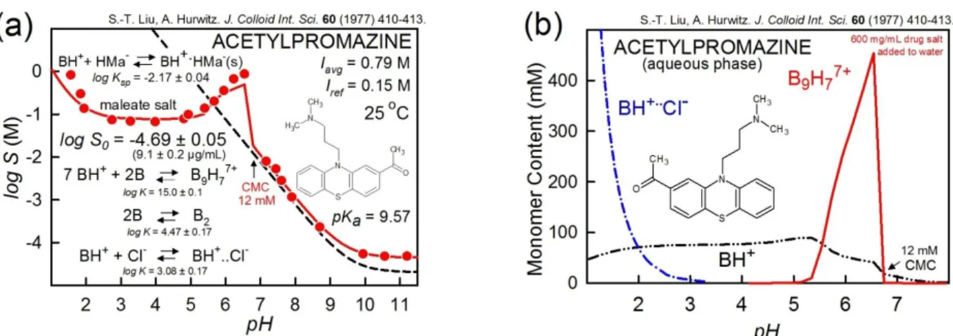
Acetylpromazine

Figure 5 is an example of the speciation of acetylpromazine maleate, a weak base with a reported critical micelle concentration of 12 mM [62]. The traditional view of simple ionic detergents is that as the concentration of added surfactant increases, monomers form until the CMC is exceeded. Further increases of the surfactant lead to the formation of micelles with aggregation numbers reaching 50 or higher, whose concentration increases, while that of the monomer remains constant. With ionizable drug molecules that have surfactant properties, the picture can be more complicated, as illustrated in Figure 5. The water-soluble sub-micellar aggregate, (B9H7)⁷⁺ best fits the “bump” portion of the logS-pH profile. The concentration of the monomer does not remain constant, and that of the aggregate formation strongly depends on pH, as shown in Figure 5b. Ion-pair interactions between chloride and the protonated form of acetylpromazine are also suggested at low pH. There may be neutral aggregates above pH 8 (Case 1b in [27]).

For additional characteristics of the fascinating properties of acetylpromazine maleate, a close inspection of the analysis detail summarized in Figures 5a and 5b, and a review of the paper by Liu and Hurwitz [62] is recommended.

Figure 5. Acetylpromazine as an example of the complexity of logS-pH profiles of surface-active molecules, suggesting that care needs to be exercised in interpreting the shapes of the solubility-pH profiles.

Summary of Issues Raised in the Case Studies

The above cases were selected as representative examples of apparently well-designed assays, which illustrate how complicated heterogeneous chemical reactions involving druglike molecules can get. There was much to consider. In several instances, it was important to know the true pKa prior to assessment of solubility- pH. When ionic strength was excessive, or when very low pH was considered, the calibration of the pH electrode required special considerations. Supersaturation had to be recognized and accordingly handled.

Distortions of the logS-pH curves due to aggregation effects had to be recognized and appropriately interpreted. There were surprises regarding the pH range over which co-precipitates (free-acid/base drug plus drug salt) could form, parting from the single-pH significance of the “pHmax” or “Gibbs pKa” ideas [42, 43]. It needs to be kept in mind that hydrates can form over long equilibration times. Mass spectrometry could be used to confirm the aggregate models derived from the computational analysis of logS-pH data. The identity of the salt forms of drug precipitates might not be obvious unless the assays were critically designed. More than one salt may form over a pH range, and sometimes the salts can overlap over a significant range of pH. Several examples of water-soluble drug-buffer complexes were suggested. In systematic testing of salts of a given drug, the salt solubility order may not be the same as the Ksp order. The interpretation of the CMC is more complicated with ionizable drugs than often recognized.

Most of the follow-up suggestions that can be made to some of the above cases could be to pursue additional corroborative investigations to confirm the presence of aggregates, to identify the stoichiometries of the solids precipitating, and the like. Unusual stoichiometry results are seldom confirmed in a different laboratory, so reliability of the models proposed can be difficult to assess. Universally, it seems that not enough attention had been devoted to the performance of the pH electrodes, particularly at very low pH. A definitive discussion of what is meant by “supersaturation” at the molecular level has not been published, as far as we are aware. It’s a term that is used frequently and has an intuitive appeal but the exact molecular mechanism has not been described. Do transient micelles and/or sub-micellar aggregates, or drug-excipient complexes, form in a supersaturated solution? Does meta-stable particle formation, or high energy interactions caused by energetic phase contacts, or increased surface tension lead to the supersaturation?

Examples of poorly designed solubility assays were not considered as case studies. Such assays outnumber

the well-designed measurements by a landslide. The goal of this commentary is to present specific recommendations that could elevate the quality of assay design, to lead to improved quality of measurements, and impart a deeper understanding of the underlying solution chemistry in the presence of drug precipitates, and how such solids can influence the interpretation of the solubility measurement.

Methods for Measuring Solubility

“Gold Standard” Shake-Flask Solubility Method

The traditional saturation shake-flask (SF) method is based on simple, easy-to perform procedures, but it is time-consuming and labor intensive. Without expensive instrumentation, SF can be conducted in any standard analytical laboratory. But to get precise and accurate solubility results, several critical experimental conditions have to be considered. When the SF method is properly performed, according to a well-designed protocol, it provides high quality data with standard deviation lower than ± 5%.

The SF method starts with the preparation of a sample suspension, the solution of the tested compound in the selected solvent (mainly in aqueous buffer - see the section below) containing a small excess of the solid.

(A large excess in the pH region where the compound converts from salt form to a free acid/base should be avoided, since the disproportionation may result in the free acid/base coating the surface of undissolved drug salt, which could result in confusing characterization of the isolated solid state material.) The volume of the suspension that should be used depends on the solubility of the sample and the concentration detection method. For majority of compounds, when the saturated solution has to be diluted for assay, 1-3 mg in 3 mL in small (10 mL) glass vial can be optimal for precise work. In such volume the pH control is easy and one can easily follow visually any changes in the vial during the equilibration. For extremely insoluble compounds, (S < 10 μg/mL) the concentration has to be measured (when using UV spectrophotometry) without dilution;

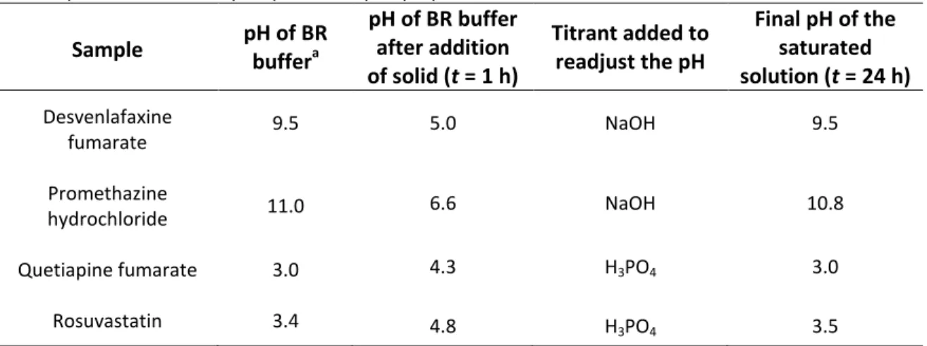
thus bigger volume of solubility suspension (1 mg solid in 15-20 mL solvent) is needed for three replicates of sampling or when 5 cm pathlength UV cell has to be used. It is a good practice to measure the pH of the solubility suspension 1 h after preparation and readjust the desired pH value if it is shifted which frequently happens when compound is applied in salt form (Table 1).

The heterogeneous system is capped and vigorously agitated (stirred) at a chosen temperature (25, 37 °C or other) in a thermostated bath for a specified time (6, 24, 48 h or longer - see the section below) until the solubility equilibrium has been reached. After that, the solid is separated from the solution by sedimentation, centrifugation or filtration (see below). Upon diluting the sample aliquots with the solvent, if necessary, the concentration of the saturated solution is measured by an appropriate method, most frequently by UV-Vis or HPLC/UV-Vis. The final pH of the saturated solution is measured.

Due to the lack of generally accepted standard way to carry out of this method, the published solubility studies show great differences in the experimental conditions used [4]. Baka et al. [3] suggested a new protocol for SF method using small excess of solid, 6 h stirring and 18 h sedimentation time and running a minimum of 3 replicates. This protocol was applied for close to 100 compounds of different structures, acid- base property, morphology, etc., and found appropriate for the precise measurement of equilibrium solubility [63].

Table 1. pH Shift of solubility suspensions upon preparation Sample pH of BR

buffer^a

pH of BR buffer after addition of solid (t = 1 h)

Titrant added to readjust the pH

Final pH of the saturated solution (t = 24 h) Desvenlafaxine

fumarate 9.5 5.0 NaOH 9.5

Promethazine

hydrochloride 11.0 6.6 NaOH 10.8

Quetiapine fumarate 3.0 4.3 H3PO4 3.0

Rosuvastatin 3.4 4.8 H3PO4 3.5

^a BR = Britton-Robinson buffer (cf., Appendix A).

CheqSol Intrinsic Solubility Method

An alternative to the shake-flask approach for measuring the intrinsic solubility of ionizable compounds is the potentiometric acid-base titration method introduced by Avdeef [42]. It is not necessary to separate the solid from the solution in the potentiometric approach (cf., Separating Solid from Saturated Solution). The intrinsic solubility is calculated from the shift between the apparent pKa (in the presence of precipitate) and the true aqueous pKa (in the absence of solid). In order to measure the true intrinsic solubility, equilibrium must be reached. This can take quite a long time, especially near the regions of complete dissolution. In order to ensure equilibrium is actually reached and in a short time, a method called CheqSol (abbreviation of

“Chasing equilibrium Solubility”) was introduced by Stuart and Box [64], and subsequently developed by Sirius Analytical (UK). The method has been validated [65] and comparison of the intrinsic solubility results measured by the SF and CheqSol techniques, when both are properly performed, shows good agreement with a weighted linear regression of logS0

SF = -0.13 + 1.00 logS0 CheqSol

(r² = 0.90, s = 0.52, n = 125) [4].

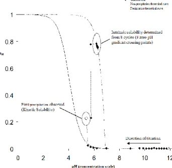
The method is based on the shift of the Bjerrum’s plot (cf., Glossary) for the titration when precipitate is present (Figure 6). The method consists of dissolving the material in water and seeking precipitation by back- titrating the resulting solution (adding measured aliquots of base or acid titrant) until first precipitation is detected. After initial precipitation of the neutral species has taken place, the solution is switched from supersaturated to subsaturated solutions and back again several times, seeking an equilibrium pH where the sample is neither further precipitating nor re-dissolving.

The method quickly pinpoints equilibrium, by advancing the pH further in the direction that it was already changing spontaneously. In contrast, the Dissolution Titration Template (DTT) potentiometric method passively allows equilibration to be reached [42]. When precipitation is occurring, the pH will change in one direction; when dissolution is occurring, pH will change in the opposite direction (see Figure 7). Therefore, by following the pH gradient, the appropriate titrant can be added to accelerate pH change in the direction of equilibration, above its ordinarily slow change. Inevitably, such titrant additions overshoot the equilibrium point, at which point the gradient will be reversed. A smaller amount of the counter titrant is then added. A change in pH of less than 0.05 is usually sufficient to reverse the direction of the pH-gradient. Such active pH

nudging, termed “chasing equilibrium,” is done as many times as necessary. The interpolated zero points of the pH-gradient indicate that the system is at equilibrium, when neither precipitation nor dissolution is observed. Each cycle between a supersaturated solution and a subsaturated one will produce a measure of the

Figure 6. Bjerrum curve (average number of associated protons (nH) vs pH) for diclofenac. The experimental data follows the theoretical curve up to the precipitation point (full circle), when it jumps onto the precipitation curve.

The direction of titration is towards the acidic region (right to left).

intrinsic solubility (Figure 7b). Usually the apparent intrinsic solubility values are distributed in a tight group around the average (true) value. If the intrinsic solubility values are not randomly distributed (like in Figure 7a), and show a systematic drift in either direction, then this means that the equilibrium has not been reached (or that a more stable polymorph can be generated), and the number of cycles is increased until the equilibrium condition is achieved. In the case of shake-flask measurements the system is allowed to shake for 6-48 h followed by long sedimentation times (cf., “Gold Standard” Shake-Flask Solubility Method), in an attempt to reach equilibrium, which is then assumed. In the CheqSol case it is easy to see if the equilibrium has been reached, and it is usually achieved for most compounds in 1-2 h (8 cycles).

Although not adapted to use auxiliary buffers, the CheqSol technique applies mass balance equations to rigorous nonlinear least squares refinement of the model based on the Henderson-Hasselbalch equation.

However, as described previously in this manuscript, a very accurate determination of the pKa of the sample is therefore needed, because the ionization constants will affect the accuracy of the concentration of the neutral species, using the Henderson-Hasselbalch relationship. Therefore a very accurate pKa needs to be measured, preferably at exactly the same conditions (temperature, ionic strength, ...).

It is not recommended to use a “predicted” value or a pKa derived from the logS-pH curve (since the Henderson-Hasselbalch equation, in many cases, may not be valid). The spread of the crossing points in CheqSol is used to determine the coefficient of variation (CV) of the mean intrinsic solubility result, which is usually <4%. The final intrinsic solubility value is calculated from an average of several separate experiments with 8 cycles per experiment, adequate to provide the intrinsic solubility value with an associated statistical reproducibility error (±SD) [1].

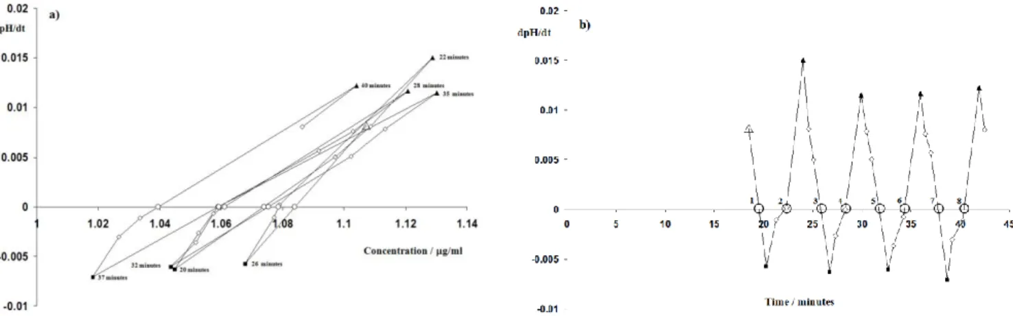
Figure 7. Chasing equilibrium of diclofenac (1 of 10 runs): the pH gradient (dpH/dt) changes from a positive value (neutral form is precipitating) in the supersaturated region to a negative one (neutral form is re-dissolving) in the subsaturated one: the rate of pH change is zero at the crossing points (○). In this run eight cycles were performed (8 crossing points). Each crossing point in plot a) corresponds to an intrinsic solubility value in b). That is, the first crossing

point, point 1 in plot a) occurs at around 20 min after the experiment has started, giving an intrinsic solubility value (first crossing point) of 1.06 μg/ml (plot b); point 2, 22 min and 1.07 μg/ml; point 3, 26 min, 1.08 μg/ml; point 4, 28 min, 1.07 μg/ml; point 5, 32 min, 1.06 μg/ml; point 6, 35 min, 1.07 μg/ml; point 7, 37 min, 1.06 μg/ml and point 8, 40

min, 1.04 μg/ml. Full triangles (▲) represent when acid titrant is added; squares (■) when base titrant is added, (◊) mean no titrant added; (○) are the crossing points, when the pH does not change, and the large empty triangle is

where the experiment starts.

The measurements are performed under inert gas (argon or nitrogen) and degassed reagents and water are used (minimal dissolved CO2). The total ionic strength, I, is kept nearly constant at 0.15 M KCl and the temperature is precisely controlled throughout (e.g., 25.0 ± 0.1 ^oC). The pH electrode is calibrated using the

“Four-Plus” method (cf., Appendix C).

Diclofenac is shown below as an example [66]. Figure 6 shows the Bjerrum curve for diclofenac. For fully dissolved diclofenac the titration curve is calculated from the pKa of diclofenac (measured previously at the same conditions as the solubility experiments) and corresponds to the continuous line in Figure 6. Aqueous pH titration was not used to determine the pKa because of precipitation problems. Instead, several titrations were performed at different concentrations of co-solvent (methanol) and the aqueous pKa was obtained by extrapolation to zero methanol concentration (Yasuda-Shedlovsky method) [27, 67-69]. The average pKa of 4.08 ± 0.04 was obtained (n=10, Iref = 0.15 M, 25 ^oC), which agrees closely with previous reported value of 3.99.

In the CheqSol method, diclofenac sodium is titrated with standardized HCl (Figure 6, high-to-low pH direction), until precipitate is turbidimetrically detected (filled circles). At this point the measurements depart suddenly from the calculated Bjerrum curve, because of the change in the amount of dissolved diclofenac. The solution is then repeatedly switched (by HCl/KOH titrant additions) from subsaturated to supersaturated states (Figure 7), until the value for the transition between the states, the solubility estimate, has converged.

The intrinsic solubility is calculated as the mean concentration of all the interpolated crossing points. The Bjerrum curve for the saturated solution is illustrated as the dot-dashed line in Figure 6. The experiment was repeated ten times and a new intrinsic solubility value is calculated as the mean of all ten converged intrinsic solubility values.

Results for one solubility determination of the sodium salt of diclofenac are illustrated in Figure 7, which represents the pH gradient against the concentration of the neutral species. Each crossing point represents the transition from supersaturated to subsaturated (or vice-versa) and so the concentration of the neutral species at zero pH gradient is the intrinsic solubility (S0) of diclofenac. All crossing points should lie close together and give essentially the same answer. The agreement in Figure 7 is excellent, with a coefficient of variation (CV) of 1.2 %. The spread of these crossing points is used to determine the CV of the mean intrinsic solubility result, and as pointed out earlier, to check if equilibrium has been reached. If the crossing points lie closely together (low CV) this means that the sample is poised at equilibrium, but if the crossing points are not in a tight bunch (high CV) or they are not randomly distributed (showing a tendency towards one single intrinsic solubility value) that means that the system needs more time to evolve towards steady state.

The diclofenac free acid was isolated by stopping the solubility experiment after eight cycles at pH 6.5. At this pH and at the end of the experiment (60 min), the solid precipitate is in equilibrium with the neutral form in solution. Differential scanning calorimetry, thermogravimetric analysis and powder X-ray diffraction were performed on this precipitate in order to fully characterize the solid. The crystal structure of this solid corresponded to the structure SIKLIH01 (Cambridge Structural Database) [70]. Characterization showed that the precipitated solid is the anhydrous form of the acid of diclofenac, space group C2/c, with an observed melting point of 180.5 °C.

Potentiometric Cycling for Polymorph Creation, [PC]²

Any solubility measurement depends on the form of the solid in equilibrium with its saturated solution. It is therefore not enough to know the solid form of the material at the beginning of the experiment. Using the CheqSol method one avoids the possibility of confounding different forms precipitating, and therefore reporting misleading data (i.e., amorphous vs crystalline, salts vs neutral forms, hydrates vs anhydrous...).

Pudipeddi and Serajuddin published a survey in 2005, showing that the difference in solubility of polymorphs is usually less than a factor of two [18]. However our results suggest that polymorphs [71] can have a considerably greater factor than this. It is therefore of vital importance to properly characterize the solid form, the solubility of which is reported, but this is rarely done in the literature.

CheqSol can be used to parse the entire Meta Stable Zone (MSZ) shown in Figure 8, starting from the first form precipitating at high supersaturation, which is the highest energy polymorph (kinetically driven), down to the last most stable form on the thermodynamic solubility saturation curve (thermodynamically driven) and achieved by cycling the system many times between supersaturation and subsaturation. This transition is normally seen as a continuous transition from the first precipitate to the most stable form, following Ostwald’s rule (see Figure 8). Metastable polymorphs encountered during this path are not, in general, stable enough to isolate and characterize, but sometimes a metastable polymorph arises during this process, being stable enough to reach a 100% of this metastable polymorph, which then can be isolated and characterized.

Nevertheless, if one continues cycling between supersaturated solution and subsaturated solution, this metastable form will evolve towards the most stable one, which will not change in form under the cycling process. It’s an advantage that these polymorph transformations can be followed in real time, when the solubility can be measured for each different form, by stopping the cycling at a specific pH, collecting the solid and characterizing it by several techniques. This cycling method has been called “Potentiometric Cycling for Polymorph Creation” [PC]².

Figure 8. Supersaturation and Oswald ripening.

This transformation can also be followed in real time using a Raman probe coupled to the potentiometric instrument enabling one to follow these phase transitions without the need of stopping the experiment and isolating the solid. This technique allows one to have a precise control of the rate of transformation of one form into the other, depending on the conditions of the experiment used.

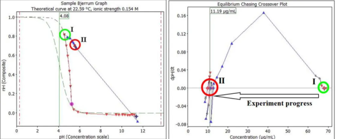
Figure 9. Bjerrum curve for sulindac depicting the first (Form I) and equilibrium cycling (Form II). Figure on the right shows the evolution of the pH gradient as the experiment progress. Note how the first precipitate form I has

a solubility around 70 μg/mL, while the most stable form, Form II, stablishes the cycling on a value around 10 μg/mL.

This approach has been applied to numerous compounds (bases, acids and zwitterions), generally obtaining the more stable polymorph; in many cases they proved to be newly-identified polymorphs [1, 66, 71-74].

Sulindac exemplifies the [PC]² approach [73]. At first the experiment produced measurements following the usual pattern of a CheqSol experiment and the readings converged on an intrinsic solubility of 70 μg/mL (Figure 9). The crystalline precipitate (Form I in Figure 9) was then isolated and characterized by powder X-ray diffraction (PXRD), Raman spectroscopy, infrared spectroscopy (IR), thermogravimetry analysis (TGA) and

differential scanning calorimetry (DSC). The powder pattern for this form (Form I) matched the pattern reported in the Cambridge Structural Database (CSD reference code DOHREX) [75]. However, it was observed that a sudden drop in solubility from about 70 to 10 μg/mL occurred after cycling for 20 min (Figures 9 and 10).

pH Versus Time

pH

Time (minutes) 5

6 7 8 9 10 11

10 20 30 40 50

Figure 10. Evolution of pH vs time for the sulindac experiment. Form I is obtained in pure form if the cycling is stopped before 20 minutes (precipitation takes place at a pH=4.5). Pure Form II is obtained when the cycling is

kept for longer times (40-50 min, pH=5.7)

0 2000 4000 6000 8000 10000 12000 14000 16000 18000 20000

0 5 10 15 20 25 30 35 40 45 50

Counts

2 Theta

Starting Material-CCDC ref. DOHREX- MATCH (Pbca)

Equilibrium Precipitate-NO MATCH / New polymorph (P2₁/c) First Precipitate-CCDC ref. DOHREX- MATCH (Pbca)

2

Figure 11 Powder X-ray diffraction of the different solid forms obtained during the sulindac [PC]² experiment. The first precipitate detected in the experiment is Form I which corresponds to the orthorhombic sulindac Pbca already described in the CCDC database (DOHREX). Form II did not match any previously reported pattern. The new polymorph of sulindac, form II, is the most stable polymorph and corresponds to the monoclinic P21/c form.

This new form has now the reference name DOHREX01 in the CCDC database.

This behavior was repeatable and setting up the conditions to cycle for more than 20 min always produced the more stable Form II with an intrinsic solubility of 10 μg/mL. This low solubility form was isolated and characterized in the same manner as Form I but in this case the powder pattern did not correspond to anything in the CSD (Figure 11). The DSC and TGA measurements confirmed that Form II has no solvent in the crystal structure, and therefore it was not simply a different hydrate of sulindac. The crystal structure of this new form (II) was solved from the powder X-ray diffraction pattern using the simulated annealing algorithm implemented in DASH [76], and refined using the Rietveld method implemented in the General Structure Analysis System [77]. The factor of seven fold between the intrinsic solubility of the original form I of sulindac

and this new more stable Form II is unusually large, but based on many other [PC]² experiments performed on different materials, a 10 fold difference is quite common. The [PC]² approach is therefore a very promising technique to measure accurately and reproducibly the intrinsic solubility of different polymorphs, since the approach is able to generate metastable and stable polymorphs. Experiment to produce the hydrate or the anhydrous form exclusively (when possible) can be designed. The application of the [PC]² technique to polymorphic systems apparently generates the most stable form of the compound, which is especially appealing to the pharmaceutical industry. By controlling the experimental conditions, also metastable forms can be obtained on purpose.

Solid State Characterization, Polymorphs, Hydrates, Cocrystals

Analysis not only of the solution, but also of the solid residue, at least at the beginning and at the end of a dissolution experiment, is often claimed to be too time-consuming, to be recommended for common use.

However, the interpretation of the results of a dissolution measurement can be misleading, if solubility refers to the wrong (or unknown) solid phase. Modern powder X-ray diffraction (PXRD) techniques make it possible to follow the composition of a solid phase directly in solution in situ, and also in high-throughput screening experiments (e.g., using instruments from Panalytical [78], or Bruker [79]). When characterizing a solid sample by PXRD, it is important not to limit the analysis by considering one or two characteristic peaks, but to analyze the whole diffraction pattern. Diffraction patterns of some polymorphs can be very similar at low values of 2 diffraction angles, so that they can be distinguished only if data are collected also at higher angles (see as an example diffraction patterns of the α, ε, ε’-polymorphs of chlorpropamide, Figure 12 [80]).

One can also use confocal Raman spectroscopy for fast analysis of the solid phase [81, 82], although Raman spectroscopy may be less sensitive for distinguishing between the polymorphs with common structural motifs than PXRD is. It is also very instructive to monitor a crystal of a selected original phase directly in solution using an optical microscope: quite often a recrystallization into another solid phase can be visually evident (see Figure 13 as an example), but that should never be taken as proof of different polymorphs since a single form can show multiple morphologies.

The following example further illustrates some of the kinds of unexpected results that may arise following solid-state characterization, which might surprise some practitioners. The differential scanning calorimetry (DSC) of a hydrochloride salt of an insoluble base (pKa  9) indicated a sharp negative peak, corresponding to the melting point of the drug salt. The salt was added in substantial excess to a neutral solution (where not the entire solid dissolved), whose pH was subsequently adjusted to 10. After 24 h, the solid was filtered out, rinsed and dried, and had its DSC run. A much lower melting point corresponding to the free base was expected.

However, the melting point actually measured by DSC was identical to the original drug salt starting material. A possible explanation is as follows. When a practically insoluble base (e.g., thioridazine) is added as a hydrochloride salt in large excess to a neutral solution, and the resultant suspension is then quickly made alkaline (pH>pKa), it is possible that the drug released from the dissolving salt particles immediately re- precipitates as the free base on the surface of the salt particles, quickly encasing them. These free-base coated particles of undissolved salt can be stable in solution. The suspension may reach a steady state after 24 h, regulated by the surface coating (which may be amorphous, or crystalline, or oil) of the practically-insoluble free base, although the suspension contains considerable undissolved crystalline salt, insulated from the

aqueous solution. The filtered solid can show a melting point corresponding to crystalline drug salt, rather than the expected free base. This example illustrates the value of solid-state characterization and the need to critically examine assay protocols.

5 10 15 20 25 30 35 40

2 Thetha

1 2 3

25 27 29 31 33 35

1 2

5 10 15 20 25 30 35 40

2 Thetha

1 2 3

25 27 29 31 33 35

1 2

2

Figure 12. Powder X-ray diffraction patterns of α- , ε’-, ε- polymorphs of chlorpropamide. Note the similarity of the patterns of the α- and ε’- polymorphs at low 2 diffraction angles; zoomed insert enlarges the diffraction

patterns of 1 and 2 at higher 2 diffraction angles, where the differences are pronounced [80].

Figure 13. Recrystallization of tolazamide polymorph II (large rhombic plates) into another tolazamide polymorph I (small elongated prisms) [83].

As seen previously (cf., “Potentiometric Cycling for Polymorph Creation”), there can be features in the solubility or dissolution curves which can suggest that the composition of the solid phase does change with time, and the results at the end of the measurements refer to another phase than at the beginning. This can be further illustrated with the example of L-glutamic acid.

L-Glutamic Acid Polymorphs

Figure 14a shows the variation of the concentration of L-glutamic acid in aqueous suspension. One can notice, that the saturated concentrations start decreasing after some time. An explanation of this phenomenon can be provided by Figure 14b, in which the relative contents of the more soluble polymorph, the α-L-glutamic, in the solid phase in contact with solution, is plotted versus time of stirring [84].

Figure 14. (a) Variation of the concentration of L-glutamic acid in aqueous solution versus time at 35 °C and 50 °C. (b) The content of the α-polymorph of L-glutamic acid in the solid sample stored in aqueous solution at 35 °C, 50 °C, 70 °C;

Data from [85].

The β-L-glutamic acid is the more stable form of L-glutamic acid [84]. The α- to β-form transition can proceed also in the solid state under humid conditions, although very slowly (being far from completion even after several months [84, 85]. Interestingly, no transition was observed on heating a dry crystal of the α-form.

In solution, when the crystals of the β-form precipitate, they deposit mainly on the surface of α-crystals, rather than as single crystals suspended in solution and the two forms can fuse into each other to such an extent, that their co-existence could be revealed only by PXRD, but not by optical microscopy [84, 85].

In Figure 15 the data from Sakata [85], processed using pDISOL-X, are presented in a comparison with similarly treated data from Lee et al. [86]. Figure 15a shows the expected parabolic-shaped logS-pH profile of L-glutamic acid, without indication of the polymorphic form. From the pDISOL-X analysis of the data, the intrinsic solubility, S0, refined to 7.5 ± 0.1 mg/mL. Figure 15b shows the result of a single-point analysis of L-glutamic acid, known to be in the β-form [85], where the refined S0 = 7.7 mg/mL. The comparable S0 values suggest that Lee et al. [86] had performed measurements on the stable β-form. It is worth pointing out that on examination of the Sakata publication [85], one encounters several shortcomings in method description, which are, unfortunately, rather common when examining published results. First, solubility has been reported in units of “g solute per 100 g water.” Given that 100 mg of NaXH.H2O plus 1 equiv. of HCl had been introduced to water, it is not clear, what is meant by “solute”, i.e., which formula weight should be used to convert to molality. The result closest to that of Lee et al. [86] suggests that “solute” refers to the zwitterion XH2 species, not salt form, NaXH.H2O, that was actually added to the solution. Such ambiguities happen quite often in the nearly 850 citations in the solubility database [4]. Clarifications are often not possible, since the authors are either no longer active, or the original experimental data cannot be located, or the authors are deceased.

Second, the final pH value was not reported [85]. For L-glutamic acid, it does not matter much, though

knowledge of the pHsat becomes important for low soluble molecules (e.g., mefenamic acid, diflunisal, fenbufen, indomethacin, clofazimine, terfenadine) [4]. Using pDISOL-X, the two calculated saturation pH values, pHsat, are 3.38 (salt) and 3.37 (zwitterion). Third, the values of ionic strength have not been reported.

Depending on which formula weight assumptions have been made, the values would be calculated as 0.54 or 0.64 M, either value well above that of normal saline.

Figure 15. The data from Sakata [85] processed using pDISOL-X in a comparison with similarly treated data from [86].

Cocrystals

Interest in pharmaceutical cocrystals emerged rapidly in the last decade [30, 87-96]. Quite often cocrystals can be formed in the physical mixtures of the two components even without any action, merely due to moisture sorption by components themselves [97], or by a polymer excipient [96, 98]. Presence of cocrystals in the drug formulation is thus possible even when not anticipated. Cocrystals are often designed and produced on purpose, to increase the solubility, or the stability, or the tabletability of an active pharmaceutical ingredient (API) [30, 92, 96, 99-104]. However, when a cocrystal is dissolved, the initially high concentration of the API in solution can drop down with time, and sometimes this happens very fast. Cocrystal solubility is sensitive to coformer concentration and pH [31]. The presence of surfactants can have a pronounced influence on the dissolution of cocrystals. Surfactants are commonly used in pharmaceutical development, in dissolution media, as formulation aids, to enhance wetting and solubility of hydrophobic drugs [105, 106], and are, of course, encountered in vivo. Whereas the micellar solubilization of single-component crystals has been thoroughly studied, micellar solubilization of cocrystals is not well understood. A key question is: how do surfactants that solubilize the drug, influence cocrystal solubility and dissolution [33, 96]? The solubility of a hydrophobic drug in aqueous solution depends on the total surfactant concentration [33]. Solubility curves of a pure drug and a cocrystal intersect at a critical stabilization concentration (CSC) point, which increases with coformer solubilization [33]. Cocrystal solubility for cocrystal R-HA in micellar solutions can be predicted from Ka and S0 values of cocrystal components (drug, coformer) and Ksp of cocrystal in blank media [28].

Cocrystal and drug solubilities converge as they approach CSC [83, 107]. Cocrystal CSC is highly sensitive to pH [108]. A key parameter, which enables the measurement of cocrystal solubility and to establish stability regions from a single experiment, is the eutectic, or transition point (Figure 16) [28]. At this point,

Scocrystal = Sdrug (cocrystal solubility in terms of drug moles); two solid phases are in equilibrium with solution;

solution composition [B]tr, [A]tr is fixed at T and pH, regardless of ratio of two solid phases [28].

Figure 16. A schematic representation for determining the eutectic, or transition point “Tr” – the point at which the “solubility of AB versus concentration of B” curve crosses the “solubility of A versus concentration of B” curve.

At this point Scocrystal = Sdrug (cocrystal solubility in terms of drug moles), and the two solid phases (AB and A) are in equilibrium with the solution. The solution composition [B]tr, [A]tr is fixed at T and pH, regardless of ratio of two

solid phases. Adapted from [28].

Carbamazepine-Nicotinamide Cocrystal

Figure 17 [108] illustrates the fast drop in the carbamazepine concentration, as indicated by the shift in the UV absorption maximum, on dissolution of a carbamazepine-nicotinamide 1:1 cocrystal in water. Two minutes after the start of the dissolution of the carbamazepine-nicotinamide cocrystal, the solid sample transforms almost completely into the carbamazepine dihydrate, with a significantly lower solubility, and the concentration of carbamazepine in solution drops. Cocrystal solid-solution equilibria are dictated by solution composition. If anhydrous carbamazepine is dissolved in the solution of nicotinamide, a 1:1 cocrystal is formed [108].

Figure 17. Transformation of a cocrystal of carbamazepine with nicotinamide into carbamazepine dihydrate on dissolution (monitored spectroscopically). Data from [108].