Comparing aggregation methods in large-scale group AHP: time for the shift to distance-based aggregation

(1)

Expert Systems With Applications 196 (2022) 116667

Available online 15 February 2022

(http://creativecommons.org/licenses/by-nc-nd/4.0/).

Comparing aggregation methods in large-scale group AHP: Time for the shift to distance-based aggregation

Szabolcs Duleba

^a^,^d^,¹^,^*

, Zsombor Sz ´ adoczki

^b^,^c^,²

aDepartment of Transport Technology and Economics, Faculty of Transportation Engineering and Vehicle Engineering, Budapest University of Technology and Economics, M˝uegyetem rkp. 3. Budapest, Hungary

bResearch Laboratory on Engineering & Management Intelligence, Institute for Computer Science and Control (SZTAKI), E¨otv¨os Lor´and Research Network (ELKH), Budapest, Hungary

cDepartment of Operations Research and Actuarial Sciences, Corvinus University of Budapest, Hungary

dInstitute of Mathematics and Informatics, University of Nyíregyh´aza, S´ost´oi u.31/b., 4400 Nyíregyh´aza, Hungary

A R T I C L E I N F O Keywords:

Group AHP Priority vector Aggregation Consensus creation Rank correlation Compatibility

A B S T R A C T

This paper aims to compare the efficiency of the conventional aggregation methods and the new, distance-based aggregation techniques in simulated and real-world group AHP cases. For the comparison, we not only applied rank correlation methods, but also examined the compatibility among the individual priority vectors of the group and the created common priority vector in the different consensus creation approaches. Results have shown that in small dimensions, both Euclidean Distance-Based Aggregation Method (EDBAM) and Aitchison Distance-Based Aggregation Method (ADBAM) outperform significantly the conventional techniques. In large dimensions, the dominance of EDBAM remains. Since the computational time of the proposed methods (especially EDBAM) is low and EDBAM maintains its efficiency in large-scale group AHP (proven by 96.000 simulation cases) in every possible dimension within the AHP domain, we can state in case of high number of evaluators, distance-based aggregation is a better approach than the conventional methods.

1. Introduction

Multi-criteria decision-making (MCDM) techniques were originally created to support the complex decisions of individuals, a few experts, or a couple of stakeholders in specific problems. As the range of applications extended, the possible number of decision-makers increased and the group approach emerged in not only theoretical, but also practical participatory problems. Recently, the number of participants in some MCDM surveys not seldom reaches thousand (Wu & Xu, 2018), mainly due to the significant role of e-democracy and social networks (Pal- omares et al., 2014) or public involvement in public service development (Duleba & Moslem, 2019). Chen & Liu (2006) created the first, widely accepted definition of a large-scale group: if more than 20 decision-makers are involved, the decision process is considered as Large-scale Group Decision-Making (LSGDM). Other researchers argued, however (Huang et al., 2009), that in the case of five participants or over, the nature of preference aggregation transforms, thus the

characteristics of LSGDM emerge. Nowadays it is a rapidly growing and very promising topic within the decision sciences but up to now, studies on LSGDM are still in its inceptive stage (Xu et al., 2018) and the available literature is very scarce in this domain. The most recent ad- vancements can be connected to Liu et al., 2019; Song & Li, 2019; Ren et al., 2020, Chai & Ngai, 2020.

Analytic Hierarchy Process (AHP) is undoubtedly one of the most popular MCDM methodologies. Like the other techniques, it is also capable of handling multiple decision-makers, Group AHP (GAHP) models are applied for problems with several participants. Although solving GAHP is almost as old as AHP itself (Acz´el & Saaty, 1983), the topic is still in the focus of researchers (Marcarelli & Squillante, 2020;

Amenta et al., 2021; Faizi et al., 2020). Owing to large-scale GAHP, most studies deal with finding the best solution to manage the transitivity and consistency of individual preferences in the aggregation procedure (Wu

& Tu, 2021) or to approximate the evaluators’ intention in scoring as

much as possible to reach accurate evaluation (Du & Shan, 2020).

* Corresponding author.

E-mail address: duleba.szabolcs@mail.bme.hu (S. Duleba).

1 ORCID: 0000-0002-2367-752X.

2 ORCID: 0000-0003-2586-5660.

Contents lists available at ScienceDirect

Expert Systems With Applications

journal homepage: www.elsevier.com/locate/eswa

https://doi.org/10.1016/j.eswa.2022.116667

Received 5 December 2020; Received in revised form 15 November 2021; Accepted 8 February 2022

(2)

A cardinal issue in GAHP is how to aggregate individual preferences and create a group consensus, which reflects the opinion of the set of participants most. The reigning techniques of aggregation are: Aggre- gation of Individual Judgements (AIJ) (Acz´el & Alsina, 1986), and Ag- gregation of Individual Preferences (AIP) (Basak & Saaty, 1993, Keeney, 2009). Both techniques apply the weighted arithmetic or weighted geometric mean of individual values, however, AIJ creates first a group matrix from the same entries of individual pairwise comparison matrices and uses the eigenvector method of AHP for this matrix afterward to derive weight vectors, while AIP computes first the individual weight vectors and then aggregates them by one of the mean calculations. Based on their comparative analysis, Ossadnik et al. (2016) stated that AIP has dominance over the AIJ technique from the aspect of preference aggregation efficiency and from the practical point of view in handling a large number of participants (which is highly relevant for the objective of our paper). Within the AIP method, there is an ongoing debate on the application of weighted arithmetic mean (AIP WAMM) and weighted geometric mean (AIP WGMM). The only existing evidence for the pri- macy of AIP WAMM is the remarkable work of Ishizaka & Labib (2011), in which they claimed that using the arithmetic mean provides more appropriate consensus creation than the geometric mean, however, they did not demonstrate this statement by simulation cases (our paper aims to contribute to this debate, please see Sub-section 3.1.). The main criticism against AIP (both forms, WAMM and WGMM) is that it could lead to a consensual priority vector which does not reflect the majority of priorities because it is subject to the influence of extreme opinions (Amenta et al., 2020). As a solution, Amenta et al. (2020) proposed a new procedure to create a common priority vector (CPVP) by a loss function minimization which is based on Euclidean norm and Euclidean distance measure. In CPVP, the saliences from the created consensual vector are minimized and thus, the distance between individual priority vectors and the common priority vector is mitigated. The authors demonstrated the new method on a real-world case study, however, simulation evidence was just remarked as further research.

Distance-based consensus creation indeed seems very promising in substituting the conventional preference aggregation techniques. The logic of finding a common priority vector in the decision space which is capable of representing all individual preference vectors by its minimum proximity to the others is reasonable. However, it is possible that other distance measures provide better consensus than the Euclidean metrics.

One of the most relevant of such different distance measures due to its widespread application in statistics, is the Aitchison distance (Aitchison et al., 2000, Stewart, 2017, Feng et al., 2020). Since the Aitchison measure is highly applicable in multi-dimensional scaling and non-Euclidean vector spaces (Quinn et al., 2018, Martín-Fern´andez et al., 2019), for determining a consensual priority vector in an n- dimensional decision space in case of n decision criteria, this metric worth investigating. Another strong argument for examining the Aitchison distance as a possible basis for preference vector aggregation is that this measure is generally used for simplexes for relative scale property (Hron et al., 2010), which is similar to the group AHP approach. Furthermore, we preliminary examined other metrics, e.g.

Chebishev and Manhattan distances, and from a compatibility point of view (between the individual vectors and the compromise vector) they significantly underperformed the Euclidean and Aitchison metrics.

The objective of our paper is to test the efficiency of different preference aggregation methods from the aspect of concordance between the individual rankings and the created consensual ranking in simulated large-scale decision-making cases. As listed above, the two techniques of the AIP method, WAMM and WGMM, furthermore two distance-based aggregations: the Euclidean Distance-Based Aggregation Method (EDBAM) and the Aitchison Distance-Based Aggregation Method (ADBAM) have been investigated. For concordance measure, first the modified form of the Kendall W calculation (Kendall, 1938) has been selected to detect the strength of the rank correlations between individual and consensual priorities. Furthermore, we applied Spearman’s

rank correlation coefficient (Kumar & Abirami, 2018), as another ordinal correlation method that deals with larger interval ([-1,1]) than the Kendall W to detect the possible negative correlation of the rankings.

Moreover, we utilized Garuti’s compatibility index (Garuti, 2017) for cardinal comparison, considering not only the similarity of the orders but also the weight scores themselves. Note that the G index was compared to Saaty’s compatibility index (based on Hadamard calculations, Saaty, 2005), and found to be more general with higher performance (Garuti, 2020). On top of that, the G index could outperform Jaccard’s index, Hilbert’s index, and the inner-vector product (IVP), thus can be considered as one of the most relevant compatibility measures between vectors.

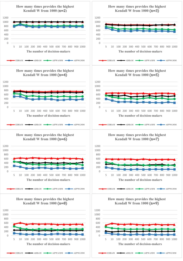
Due to the high difficulty of generating matrices with acceptable consistency ratio and the complexity of conducting a large number of simulations in the case of Spearman and Garuti calculations, we examined a smaller number of simulated matrices in this phase. In the large- scale procedure based on Kendall W, we randomly generated normalized vectors in different dimensions (following the AHP characteristics and the rule of Saaty from two dimensions to nine dimensions - because of Saaty’s concept (Saaty, 1994) on the maximum size of pairwise comparison matrices 9×9 to keep the consistency of evaluations) and examined the cases of five, ten, 100, 200,…, 1000 decision-makers.

Afterwards, we computed the consensual group priority vector by the four different aggregation techniques and calculated the Kendall W value to measure each rank correlation. We repeated it 1000 times for each combination of dimensions and number of decision-makers. Alto- gether 8x12.000 =96.000 simulation cases were examined as we tested the eight different dimensions for 12 different evaluator numbers with the repetition of 1000 times, and for each case, four different Kendall W is computed by AIP WAMM, AIP WGMM, EDBAM and ADBAM aggregation methods. The whole analysis is demonstrated in Section 3.

In the next phase of simulations, we followed the original approach of AHP, and generated random pairwise comparison matrices in different dimensions using merely the values of the Saaty-scale and considering the consistency threshold of 10% for the Consistency Ratio in case of at most 6 alternatives (criteria) and 20% for even larger in- stances. From 2×2 up to 9×9 sized matrices, 10 participants were assumed, their evaluations were derived by the eigenvector method and these weight vectors were aggregated by EDBAM, ADBAM, AIP WAMM, AIP WGMM and CPVP methods. The results were compared by both Spearman’s rank correlation coefficient and G compatibility index.

Thus, for the first time in the literature of decision science and multi- criteria decision-making, we can compare the efficiency of the examined different aggregation approaches and recommend the most appropriate for large-scale group AHP decision-making. Moreover, we apply all examined aggregation methods on real-world data gained from a survey conducted in a Turkish city, Mersin, on citizen preferences towards public transport development issues. The preferences of ten evaluators are highlighted on five attributes and we demonstrate the difference in determining the common priority vectors and the different concor- dances of the common priority vectors respect to the individual preference rankings. Different Kendall W values are computed from the case study which supports the simulation results and the initial idea: it is time for shift to distance-based methods in aggregating individual preferences in group AHP.

The remainder of the paper is organized as follows. We introduce the AHP methodology in detail, along with the studied different aggregation methods and the measurements used in the comparisons in Section 2.

The large-scale simulation results and the analysis of the gained infor- mation can be found in Sub-section 3.1. More specific simulated group AHP examples are presented in Sub-section 3.2. using both ordinal and cardinal indicators. We present the above-mentioned real-world numerical example in detail, based on the previously conducted group AHP survey in Sub-section 3.3. Finally, we draw some conclusions and make suggestions to the future appliers of the aggregation methods in Section 4.

(3)

2. Methodology

As we mentioned in the Introduction, the application of the Analytic Hierarchy Process is indeed widespread. It is based on the Pairwise Comparison Matrices (PCMs), which can be used both for determining the weights of the different criteria and for the rating of alternatives according to a criterion. The n×n matrix A= [aij]is a PCM if it is pos- itive (aij>0 for ∀i and j) and reciprocal (aji=1/aij for ∀i and j). Its general element aij shows, how many times item i is better/larger/more important than element j. A PCM is said to be consistent if and only if aik=aijajk for ∀i,j,k,1≤i,j,k≤n, and it is inconsistent in all other cases.

In a practical decision problem the matrix is most likely to be inconsistent, however there can be significant differences in the degree of

consistency that can be measured by the Consistency Ratio (CR):

CR=CI RI,

where RI is the average CI value of randomly generated PCMs of the same size, while:

CI=λmax− n n− 1 ,

where CI denotes the Consistency Index and λmax is the largest eigenvalue of the examined PCM. In AHP the acceptable consistency degree is generally indicated by CR<0.1.

Let us denote the number of evaluators in a group decision-making

(4)

problem by m, let w^(k)=

(w⁽₁^k⁾,w⁽₂^k⁾,⋯,w⁽n^k⁾

)_T

be the individual priority vector for decision-maker k (w^(k)_i >0 for ∀i=1,2,⋯,n and ∑_n

i=1w^(k)_i =1 for ∀k=1,2,⋯,m). Besides the two proposed distance-based preference aggregation techniques, we also include two variants of the well-known

Aggregation of Individual Preferences (AIP) as a benchmark in this paper.

As for the AIP Weighted Arithmetic Mean Method (WAMM), the consensual preference vector w^(A)is computed as the weighted arithmetic mean of the individual priorities:

0 200 400 600 800 1000 1200

5 10 100 200 300 400 500 600 700 800 900 1000 The number of decision-makers

How many times provides the highest Kendall W from 1000 ( )

EDBAM ADBAM AIPWAMM AIPWGMM

0 200 400 600 800 1000 1200

How many times provides the highest Kendall W from 1000

0 200 400 600 800 1000 1200

Fig. 1. Large-scale simulation results for the different aggregation methods.

(5)

w^(A)_i =∑^m

k=1

akw^(k)_i ,i=1,2,⋯,n.

where ak is the weight of evaluator k and ∑_m

k=1ak =1. In case of the AIP Weighted Geometric Mean Method (WGMM), the common preference vector w⁽^G⁾is obtained by calculating the weighted geometric mean of the individual priorities:

w^(G)_i =

∏_m

k=1

( w^(k)_i

)_a_k

∑_n

i=1

∏_m

k=1

( w^(k)_i

)_a_k,i=1,2,⋯,n.

where ∑_m

k=1ak=1 as before.

Later, in the presentation of more specific examples, we also include the CPVP method (Amenta et al., 2020) in our examinations, which is based on the optimization of a loss function defined as follows.

min

λk,qL(q,λk) =∑^m

k=1

ak‖Wk− λkqq^T‖_F²

Where ‖.‖_Fdenotes the Frobenius norm (that is basically the matrix version of the Euclidean distance), ∑_m

k=1ak=1 as before and Wk is defined by:

Wk=λkqkq^T_k

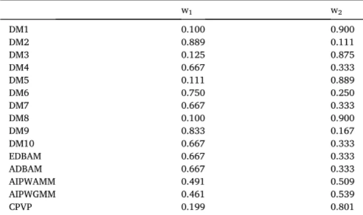
where λk is the principal eigenvalue of the PCM related to evaluator k, while qk is the eigenvector connected to the principal eigenvalue. In order to obtain a numerical solution, one should use Algorithm 1 of Amenta et al., 2020, as the optimization is needed in two variables, which affect each other. This method is the closest to our proposals in its logic, thus it is important to include it in the paper, however, in the first, Table 1

The ten normalized simulated preference vectors and the related aggregated priority vectors for n=2.

w1 w2

DM1 0.100 0.900

DM2 0.889 0.111

DM3 0.125 0.875

DM4 0.667 0.333

DM5 0.111 0.889

DM6 0.750 0.250

DM7 0.667 0.333

DM8 0.100 0.900

DM9 0.833 0.167

DM10 0.667 0.333

EDBAM 0.667 0.333

ADBAM 0.667 0.333

AIPWAMM 0.491 0.509

AIPWGMM 0.461 0.539

CPVP 0.199 0.801

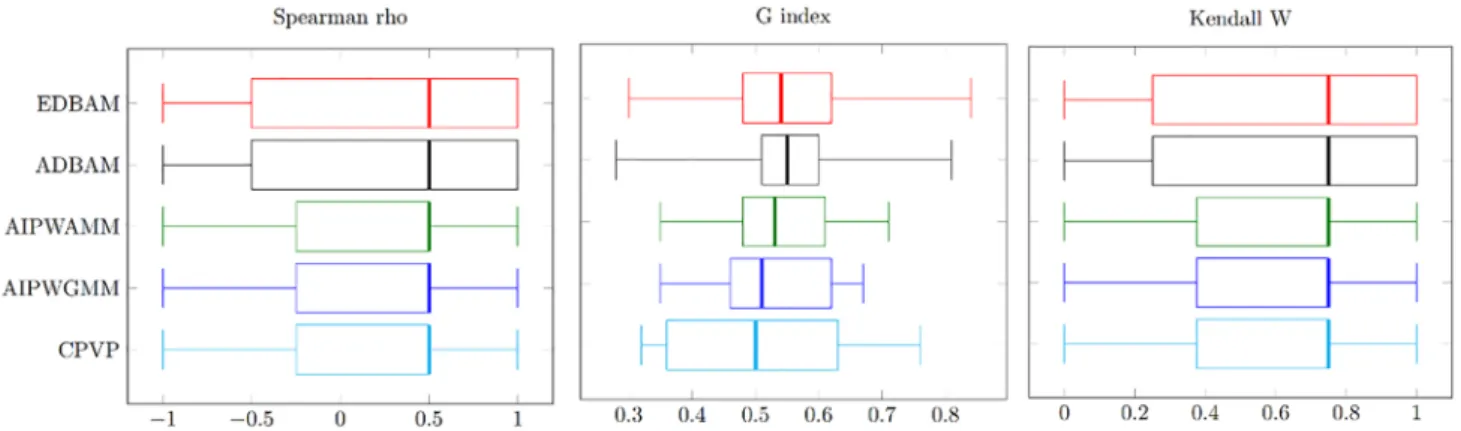
Table 2

Basic statistics of the G index, Spearman’s rank correlation coefficient and Kendall W of the aggregated priority vectors respect to the individual preference vectors for n=2. Please see Fig. 2 for the graphical presentation.

EDBAM ADBAM AIPWAMM AIPWGMM CPVP

Average G index 0.640 0.640 0.551 0.542 0.518

Average Spearman

rho 0.2 0.2 −0.2 −0.2 − 0.2

Average Kendall W 0.6 0.6 0.4 0.4 0.4

St. dev. G index 0.320 0.320 0.111 0.089 0.106 St. dev. Spearman

rho 1.033 1.033 1.033 1.033 1.033

St. dev. Kendall W 0.516 0.516 0.516 0.516 0.516

Fig. 2. Box-plots of the G index, Spearman’s rank correlation coefficient and Kendall W of the aggregated priority vectors respect to the individual preference vectors for n=2.

Table 3

The ten normalized simulated preference vectors and the related aggregated priority vectors for n=3. Please see Fig.3 for the graphical presentation.

w1 w2 w3

DM1 0.073 0.671 0.256

DM2 0.705 0.211 0.084

DM3 0.674 0.226 0.101

DM4 0.117 0.806 0.077

DM5 0.489 0.067 0.444

DM6 0.537 0.364 0.099

DM7 0.078 0.750 0.171

DM8 0.167 0.094 0.740

DM9 0.600 0.300 0.100

DM10 0.063 0.458 0.479

EDBAM 0.446 0.359 0.195

ADBAM 0.429 0.392 0.179

AIPWAMM 0.350 0.395 0.255

AIPWGMM 0.327 0.418 0.255

CPVP 0.227 0.580 0.192

Table 4

Basic statistics of the G index, Spearman’s rank correlation coefficient and Kendall W of the aggregated priority vectors respect to the individual preference vectors for n=3. Please see Fig. 3 for graphical presentation.

Average G index 0.555 0.552 0.533 0.530 0.511 Average Spearman

rho 0.25 0.25 0.2 0.2 0.2

rho 0.791 0.791 0.632 0.632 0.632

St. dev. Kendall W 0.395 0.395 0.316 0.316 0.316

(6)

large-scale phase of the simulations we only concentrate on the benchmark techniques (AIP WAMM and AIP WGMM) in the comparisons.

2.1. Distance-based preference aggregation techniques

The main reason for the preference aggregation methods that we propose is to look for the closest vector to the individual priority vectors according to a certain metric. Regarding the Euclidean Distance-Based Aggregation Method (EDBAM), the group preference vector w^(E)is the solution of the following formula normalized to one:

argminf(x)

Where x∈Rⁿand f(x)is defined as follows:

f(x) =∑^m

k=1

(ak∙dE(w^(k),x))

Where dE

(w^(k),x)

=

̅̅̅̅̅̅̅̅̅̅̅̅̅̅̅̅̅̅̅̅̅̅̅̅̅̅̅̅̅̅̅̅̅̅̅̅̅

∑_n

i=1

(w⁽_i^k⁾− xi

)₂

√

is the Euclidean distance, and ∑_m

k=1ak=1 as before. Thus, we determine the vector in Rⁿthat is the nearest one to the individual priority vectors and then normalize it to one.

In case of the Aitchison Distance-Based Aggregation Method (ADBAM) we follow the same steps except that we are minimizing according to the Aitchison distance,dA(., .):

dA

(w^(k),x)

=

̅̅̅̅̅̅̅̅̅̅̅̅̅̅̅̅̅̅̅̅̅̅̅̅̅̅̅̅̅̅̅̅̅̅̅̅̅̅̅̅̅̅̅̅̅̅̅̅̅̅̅̅̅̅̅̅̅̅̅̅̅̅̅̅̅̅̅̅̅̅̅̅

∑ⁿ

i=1

[ log

( w^(k)_i g(w^(k))

)

− log ( xi

g(x) ) ]2

√√

Where g(w⁽^k⁾)and g(x)denote the geometric mean of the respective vectors and log(.)is the function of natural logarithm.

In order to find the solution of the optimization problems connected to the distance-based methods, we use the method of Nelder & Mead (1965), which is a robust technique and uses only function values. In our simulations we apply the R implementation of this method, which can be seen as an algorithm below.

2.2. The comparison of the techniques

As for the comparison of the different preference aggregation methods, from the several techniques that can measure the degree of consensus, we examine various indicators. The first one is the Kendall coefficient of concordance (Kendall W) calculation, which provides an overall measure of agreement in ranking, as the prioritization of the alternatives or criteria is our major goal. In our case, the appropriate procedure is to supplement the rankings provided by the individual decision-makers with the consensual priority ranking calculated with the help of one of the aforementioned methods, and examine the strength of concordance. Kendall W has the common [0,1]range, and the higher its value is, the stronger the correlation in ranking. Thus, the technique that provides the highest Kendall coefficient of concordance for a given dataset has the strongest correlation in ranking with the preferences of the evaluators, accordingly, it can be considered as the best in that case. This way it is a suitable tool to compare the different preference aggregation methods with each other. However, keep in mind that not the value of the Kendall W itself, but the differences between the provided measures is the key, as the coefficient quantifies the concordance between the different individual evaluators as well. The Kendall W is a non-parametric statistic that can be calculated as follows.

Let ri,k be the rank given to item i by decision-maker k, and Ri be the aggregated ranking of element i:

Table 5

w1 w2 w3 w4

DM1 0.081 0.074 0.397 0.448

DM2 0.174 0.051 0.520 0.255

DM3 0.108 0.095 0.704 0.093

DM4 0.259 0.508 0.056 0.177

DM5 0.061 0.535 0.302 0.102

DM6 0.472 0.339 0.106 0.082

DM7 0.178 0.400 0.086 0.336

DM8 0.249 0.203 0.051 0.497

DM9 0.531 0.090 0.094 0.285

DM10 0.043 0.699 0.174 0.084

EDBAM 0.220 0.330 0.203 0.248

ADBAM 0.231 0.313 0.189 0.268

AIPWAMM 0.216 0.299 0.249 0.236

AIPWGMM 0.220 0.288 0.231 0.261

CPVP 0.178 0.432 0.202 0.188

Table 6

Basic statistics of the G index, Spearman’s rank correlation coefficient and Kendall W of the aggregated priority vectors respect to the individual preference vectors for n=4. Please see Fig. 4 for graphical presentation.

Average G index 0.551 0.551 0.542 0.544 0.547

Average Spearman

rho 0.06 0.06 0.02 0.04 0.02

rho 0.640 0.640 0.649 0.617 0.649

St. dev. Kendall W 0.320 0.320 0.325 0.308 0.325

(7)

Ri=∑^m

k=1

ri,k,i=1,2,⋯,n

Let us denote the mean of the aggregated ranking by R:

R=m(n+1) 2

The sum of squares deviation statistic of the aggregated rankings defined by the following:

S=∑ⁿ

i=1

(Ri− R)²

Finally, the Kendall coefficient of concordance can be obtained from the formula below:

W= 12S m²(n³− n)

When ties occur, W has to be modified by the following correction factor:

Tk=∑^g^k

i=1

(t³_i− ti

)

wheregkis the number of groups of ties for decision-makerk and tiis the number of tied ranks in thei th group of tied ranks. In this case the corrected Kendall coefficient of concordance can be calculated as follows.

W=12∑_n

i=1(Ri)²− 3m²n(n+1)² m²(n³− n) − m∑_m

k=1Tk

Table 7

w1 w2 w3 w4 w5

DM1 0.429 0.073 0.102 0.341 0.055

DM2 0.152 0.038 0.127 0.100 0.582

DM3 0.040 0.081 0.088 0.456 0.336

DM4 0.317 0.171 0.372 0.042 0.097

DM5 0.038 0.067 0.134 0.549 0.211

DM6 0.034 0.135 0.199 0.048 0.583

DM7 0.500 0.309 0.044 0.082 0.065

DM8 0.066 0.515 0.052 0.255 0.112

DM9 0.389 0.224 0.272 0.065 0.050

DM10 0.200 0.404 0.211 0.043 0.142

EDBAM 0.162 0.329 0.127 0.145 0.238

ADBAM 0.152 0.271 0.127 0.145 0.305

AIPWAMM 0.157 0.279 0.153 0.151 0.259

AIPWGMM 0.162 0.244 0.145 0.149 0.300

CPVP 0.144 0.352 0.117 0.132 0.255

Table 8

Basic statistics of the G index, Spearman’s rank correlation coefficient and Kendall W of the aggregated priority vectors respect to the individual preference vectors for n=5.

Average G index 0.514 0.516 0.512 0.514 0.499

Average Spearman

rho 0.01 0.02 −0.02 −0.01 − 0.06

Average Kendall W 0.490 0.485 0.500 0.485 0.490 St. dev. G index 0.088 0.072 0.069 0.067 0.094 St. dev. Spearman

rho 0.402 0.380 0.419 0.380 0.402

St. dev. Kendall W 0.201 0.190 0.209 0.190 0.201

Table 9

w1 w2 w3 w4 w5 w6

DM1 0.029 0.452 0.042 0.101 0.136 0.241

DM2 0.100 0.316 0.065 0.042 0.027 0.450

DM3 0.506 0.104 0.054 0.202 0.092 0.042

DM4 0.086 0.034 0.295 0.050 0.086 0.449

DM5 0.034 0.095 0.275 0.335 0.161 0.100

DM6 0.384 0.025 0.329 0.112 0.054 0.096

DM7 0.092 0.061 0.045 0.285 0.218 0.299

DM8 0.062 0.096 0.124 0.555 0.133 0.030

DM9 0.328 0.044 0.083 0.047 0.224 0.274

DM10 0.413 0.253 0.028 0.058 0.192 0.057

EDBAM 0.157 0.156 0.124 0.275 0.131 0.158

ADBAM 0.116 0.161 0.134 0.304 0.114 0.172

AIPWAMM 0.146 0.165 0.145 0.254 0.126 0.164 AIPWGMM 0.115 0.163 0.144 0.286 0.115 0.176

CPVP 0.144 0.157 0.138 0.286 0.119 0.156

Table 10

rho 0.189 0.194 0.149 0.189 0.171

rho 0.250 0.313 0.311 0.416 0.311

St. dev. Kendall W 0.125 0.157 0.155 0.208 0.155

(8)

We also use the well-known Spearman’s rank correlation coefficient (Spearman rho) that is applicable for two vectors, given by the formula below:

ρ=1− 6∑_n

i=1d²_i n³− n

where di is the difference of the rank of element i for the examined vectors. When there are ties in the ranks the equation is modified as follows:

ρ=cov(r1,r2) σr1σr2

where r1 and r2 denote the rankings defined by the first and second examined vectors, cov(., .)is the covariance of two variables, while σ is

the standard deviation of a variable. This indicator’s value is in the range [ − 1,1], thus it can also show the complete disagreement between two preference vectors, compared to the Kendall W measurement.

As for the cardinal indicators, we use Garuti’s compatibility index (G index) (Garuti, 2020) that is also applicable for two preference vectors and defined as follows.

G=1 2

∑ⁿ

i=1

min (

w⁽¹⁾_i ,w⁽²⁾_i )

max (

w⁽¹⁾_i ,w⁽²⁾_i

)(w⁽¹⁾_i +w⁽²⁾_i )

Where w⁽_i¹⁾and w⁽_i²⁾denote the i th element of the first and second examined vectors. The higher the G index, the more compatible the two respective vectors are. It is important to focus on both ordinal and cardinal measurements as there can be large contrasts between the results according to these indicators, because their calculation method and logic is different, indeed.

In Sub-section 3.2. we compute the average Spearman rho-s and G indices of the individual preference vectors respect to the given aggregated vectors and compare these averages for the aggregation methods to find the best techniques.

3. Results

3.1. Large-scale preference vector simulations

In order to compare the performance of the different preference aggregation techniques in Large-scale Group Decision-Making problems, we completed a wide range of numerical simulations. We examined two to nine dimensional preference vectors (n), while the studied number of evaluators (m)were 5, 10, 100, 200, …, 1000. The simulation for a given Table 11

w1 w2 w3 w4 w5 w6 w7

DM1 0.497 0.255 0.051 0.043 0.083 0.041 0.030 DM2 0.023 0.034 0.237 0.052 0.509 0.078 0.066 DM3 0.024 0.244 0.056 0.262 0.140 0.055 0.219 DM4 0.223 0.065 0.057 0.214 0.063 0.053 0.326 DM5 0.064 0.036 0.303 0.071 0.360 0.081 0.084 DM6 0.231 0.052 0.060 0.398 0.027 0.069 0.163 DM7 0.062 0.273 0.076 0.299 0.022 0.114 0.153 DM8 0.054 0.163 0.212 0.051 0.415 0.042 0.062 DM9 0.052 0.213 0.099 0.064 0.127 0.136 0.309 DM10 0.414 0.034 0.163 0.057 0.042 0.097 0.193 EDBAM 0.211 0.096 0.116 0.120 0.227 0.147 0.083 ADBAM 0.217 0.103 0.098 0.125 0.238 0.140 0.081 AIPWAMM 0.203 0.101 0.129 0.123 0.213 0.135 0.096 AIPWGMM 0.208 0.108 0.112 0.128 0.217 0.132 0.095 CPVP 0.228 0.089 0.105 0.109 0.255 0.136 0.078

Table 12

Average G index 0.523 0.522 0.517 0.520 0.495

Average Spearman

rho 0.196 0.232 0.096 0.232 0.157

rho 0.377 0.314 0.460 0.377 0.377

St. dev. Kendall W 0.188 0.157 0.230 0.188 0.188

Table 13

w1 w2 w3 w4 w5 w6 w7 w8

DM1 0.088 0.080 0.063 0.024 0.143 0.351 0.051 0.199

DM2 0.090 0.024 0.016 0.230 0.071 0.038 0.224 0.307

DM3 0.191 0.082 0.024 0.149 0.030 0.317 0.044 0.163

DM4 0.033 0.319 0.051 0.103 0.291 0.141 0.039 0.023

DM5 0.403 0.099 0.031 0.091 0.018 0.237 0.079 0.042

DM6 0.167 0.051 0.184 0.298 0.018 0.078 0.018 0.186

DM7 0.237 0.318 0.059 0.090 0.023 0.129 0.016 0.129

DM8 0.030 0.179 0.154 0.357 0.038 0.036 0.176 0.029

DM9 0.097 0.028 0.167 0.024 0.066 0.136 0.197 0.286

DM10 0.045 0.072 0.108 0.019 0.368 0.085 0.176 0.127

EDBAM 0.141 0.120 0.085 0.136 0.096 0.164 0.099 0.159

ADBAM 0.157 0.123 0.083 0.120 0.078 0.189 0.089 0.161

AIPWAMM 0.138 0.125 0.086 0.138 0.107 0.155 0.102 0.149

AIPWGMM 0.144 0.126 0.091 0.127 0.086 0.170 0.099 0.156

CPVP 0.166 0.122 0.077 0.134 0.084 0.178 0.089 0.150

Table 14

rho 0.248 0.245 0.240 0.240 0.233

rho 0.433 0.366 0.445 0.334 0.433

St. dev. Kendall W 0.216 0.183 0.222 0.167 0.216

(9)

(n,m)pair consists of the steps detailed below.

Algorithm 2.: Process of the simulation Input: (n,m)pair of parameters.

Output: The number of times when a method provided the highest Kendall W of 1000 cases for AIP WAMM, AIP WGMM, EDBAM, and ADBAM.

1. Generate m different n-dimensional random vectors, which are normalized to one (individual preference vectors).

2. Apply the AIP WAMM, AIP WGMM, EDBAM and ADBAM methods on the individual vectors (detailed in Section 2) resulting in the following priority vectors:

wÂIPWAMM, wÂIPWGMM,wÊDBAMand wÂDBAM.

3. Collect the rankings provided by the individual decision-makers and by the consensual priority ranking calculated according to the appropriate method in the following matrices: MÂIPWAMM, MÂIPWGMM,MÊDBAMand MÂDBAM.

4. The tie-corrected Kendall coefficient of concordance measure is calculated for the four matrices and those methods that provide the highest Kendall W are saved.

5. Steps 1–4 are repeated 1000 times.

Return: A (4-dimensional) vector contains the number of times when AIP WAMM, AIP WGMM, EDBAM, and ADBAM provided the highest Kendall W of 1000 cases.

Based on this procedure, we examined a total of 8×12000=96000 cases, and the efficiency of the preference aggregation techniques according to the dimensions of the priority vectors and the number of Table 15

w1 w2 w3 w4 w5 w6 w7 w8 w9

DM1 0.045 0.072 0.052 0.043 0.046 0.392 0.154 0.023 0.173

DM2 0.041 0.187 0.051 0.404 0.071 0.028 0.127 0.076 0.016

DM3 0.094 0.053 0.226 0.315 0.029 0.016 0.026 0.118 0.123

DM4 0.135 0.177 0.020 0.070 0.023 0.030 0.148 0.325 0.071

DM5 0.225 0.235 0.135 0.158 0.028 0.088 0.076 0.035 0.019

DM6 0.233 0.046 0.165 0.172 0.052 0.015 0.055 0.094 0.168

DM7 0.333 0.036 0.127 0.020 0.098 0.045 0.023 0.269 0.050

DM8 0.225 0.235 0.135 0.158 0.028 0.088 0.076 0.035 0.019

DM9 0.233 0.046 0.165 0.172 0.052 0.015 0.055 0.094 0.168

DM10 0.333 0.036 0.127 0.020 0.098 0.045 0.023 0.269 0.050

EDBAM 0.207 0.107 0.136 0.158 0.050 0.056 0.067 0.122 0.096

ADBAM 0.215 0.105 0.145 0.148 0.059 0.045 0.075 0.122 0.086

AIPWAMM 0.190 0.112 0.120 0.153 0.052 0.076 0.076 0.134 0.086

AIPWGMM 0.206 0.115 0.134 0.136 0.062 0.057 0.082 0.127 0.081

CPVP 0.219 0.103 0.130 0.144 0.057 0.048 0.063 0.155 0.080

Table 16

Average G index 0.599 0.599 0.582 0.588 0.593

Average Spearman

rho 0.380 0.382 0.377 0.375 0.375

rho 0.421 0.445 0.420 0.436 0.420

St. dev. Kendall W 0.210 0.222 0.210 0.218 0.210

Table 17

The normalized AHP scores of ten individual respondents in the public transport development survey.

Approachability Directness Time availability Speed Reliability

Evaluator1 0.2406 0.2940 0.1408 0.1388 0.1858

Evaluator2 0.2575 0.1448 0.2244 0.1246 0.2488

Evaluator3 0.2886 0.0717 0.1257 0.2535 0.2604

Evaluator4 0.1853 0.2881 0.1707 0.1332 0.2227

Evaluator5 0.2160 0.4059 0.0609 0.2129 0.1043

Evaluator6 0.0524 0.3127 0.2296 0.3135 0.0918

Evaluator7 0.0615 0.1586 0.2587 0.3635 0.1577

Evaluator8 0.2930 0.0721 0.2771 0.1625 0.1953

Evaluator9 0.2608 0.2143 0.1311 0.1546 0.2393

Evaluator10 0.2708 0.2189 0.2510 0.1739 0.0854

Table 18

The normalized consensual priority vector of EDBAM.

EDBAM

Approachability 0.2276

Directness 0.2234

Time availability 0.1792

Speed 0.1776

Reliability 0.1922

Kendall W 0.1521

Table 19

The calculation of Kendall W in case of EDBAM.

Criteria Rank of

Evaluator1 … Rank of

EDBAM Ri (Ri− R)²

Approachability 2 … 1 23 100

Directness 1 … 2 30 9

Time

availability 4 … 4 38 25

Speed 5 … 5 40 49

Reliability 3 … 3 34 1

n =5 m =11 S =

184 R =33 W =0.1521

Table 20

The normalized consensual priority vector of ADBAM.

ADBAM

Approachability 0.2269

Directness 0.2215

Time availability 0.1764

Speed 0.1761

Reliability 0.1990

Kendall W 0.1521