Feedforward attractor targeting for non- linear oscillators using a dual-frequency driving technique

(1)

linear oscillators using a dual-frequency driving technique

Cite as: Chaos 30, 073123 (2020); https://doi.org/10.1063/5.0005424

Submitted: 02 March 2020 . Accepted: 15 June 2020 . Published Online: 14 July 2020 F. Hegedűs , P. Krähling, M. Aron , W. Lauterborn , R. Mettin, and U. Parlitz

ARTICLES YOU MAY BE INTERESTED IN

Terminating transient chaos in spatially extended systems

Chaos: An Interdisciplinary Journal of Nonlinear Science 30, 051108 (2020); https://

doi.org/10.1063/5.0011506

Identifying edges that facilitate the generation of extreme events in networked dynamical systems

doi.org/10.1063/5.0002743

Asymptotic estimates of SARS-CoV-2 infection counts and their sensitivity to stochastic perturbation

doi.org/10.1063/5.0008834

(2)

Feedforward attractor targeting for non-linear oscillators using a dual-frequency driving

technique

Cite as: Chaos30, 073123 (2020);doi: 10.1063/5.0005424 Submitted: 2 March 2020·Accepted: 15 June 2020·

Published Online: 14 July 2020 View Online Export Citation CrossMark

F. Heged ˝us,^1,a) P. Krähling,^1,b)M. Aron,^2,c) W. Lauterborn,^3,d) R. Mettin,^3,e)and U. Parlitz^2,f)

AFFILIATIONS

1Department of Hydrodynamic Systems, Faculty of Mechanical Engineering, Budapest University of Technology and Economics, M˝uegyetem rakpart 3, H-1111 Budapest, Hungary

2Research Group Biomedical Physics, Max Planck Institute for Dynamics and Self-Organization, Am Fassberg 17, D-37077 Göttingen, Germany and Institut für Dynamik komplexer Systeme, Georg-August-Universität Göttingen, Friedrich-Hund-Platz 1, D-37077 Göttingen, Germany

3Drittes Physikalisches Institut, Georg-August-Universität Göttingen, Friedrich-Hund Platz 1, D-37077 Göttingen, Germany

a)Author to whom correspondence should be addressed:fhegedus@hds.bme.hu.URL:www.gpuode.com

b)krahling.peter@gmail.com

c)marcel.aron@ds.mpg.de

d)werner.lauterborn@phys.uni-goettingen.de

e)robert.mettin@phys.uni-goettingen.de

f)ulrich.parlitz@ds.mpg.de

ABSTRACT

A feedforward control technique is presented to steer a harmonically driven, non-linear system between attractors in the frequency–amplitude parameter plane of the excitation. The basis of the technique is the temporary addition of a second harmonic component to the driving. To illustrate this approach, it is applied to the Keller–Miksis equation describing the radial dynamics of a single spherical gas bubble placed in an infinite domain of liquid. This model is a second-order, non-linear ordinary differential equation, a non-linear oscillator. With a proper selection of the frequency ratio of the temporary dual-frequency driving and with the appropriate tuning of the excitation amplitudes, the trajectory of the system can be smoothly transformed between specific attractors; for instance, between period-3 and period-5 orbits. The transformation possibilities are discussed and summarized for attractors originating from the subharmonic resonances and the equilibrium state (absence of external driving) of the system.

Published under license by AIP Publishing.https://doi.org/10.1063/5.0005424

The governing equations of many physical phenomena are non- linear. One of the main consequences of non-linearity is the existence of various types of stable solutions (e.g., equilibrium, periodic, quasiperiodic, or chaotic) over the parameter space of the system. At a given parameter combination, many such stable states might co-exist exhibiting multi-stability. From an appli- cation point of view, the features mentioned above can cause unpredictable behavior as the different stable states usually rep- resent different system performances. Therefore, it is mandatory to be able to drive a system to a desirable state. The control tech- nique presented in this paper performs this task for periodic solu- tions of harmonically excited non-linear oscillators. The main strength of the method is that direct attractor selection is possible

without the application of feedback on the system. Although the control procedure is demonstrated only for a specific sys- tem (Keller–Miksis equation), the generalization of the principles of the technique for other non-linear systems can significantly broaden its applicability to a large number of scientific fields in the future, for instance, in mechanical engineering, chemistry, laser physics, fluid dynamics, or social sciences, to name a few.

I. INTRODUCTION

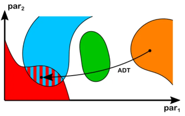
In the parameter space of many non-linear systems, different domains of attractors occur,^1–12 as illustrated in Fig. 1. These domains can overlap in certain parameter regions representing

(3)

FIG. 1. Sketch of domains of attractors in a two-dimensional parameter space.

The different colors represent different families of continuously connected attractors. The abbreviation ADT stands for theAttractor Domain Targetingtechnique.

multi-stability. The behavior of the system is usually different from domain to domain. For instance, chemical reactions can have different chemical yields for different attractors.^1,11,13In cardiac models, the different stable states can represent normal cardiac rhythm or lethal arrhythmia.^14–17In the case of a large number of coupled systems (e.g., power grids¹⁸), two stable states may display the difference between synchronous and asynchronous behavior.^19–22 Therefore, the ability to drive a system between domains of stable states is important to maintain and control its performance. As the domains do not necessarily overlap each other, this is an extended concept of control of multi-stability.^23–26The proposed method that is capable of driving a system smoothly between stable states having distinct parameter sets is calledAttractor Domain Targeting (ADT) technique throughout the present paper. The arrow between the two black dots inFig. 1represents this method. Note that this specific problem is a non-trivial task as the attractors represented by the two black dots may not be connected by a continuous transformation; in addition, in this example, the “blue” attractor may co-exist with the

“red” one.

The main aim of this study is to present an ADT technique that works for harmonically driven non-linear oscillators. It is capable of smoothly steering such a system between periodic domains of attractors in the amplitude–frequency parameter plane of the excitation by temporarily adding a second harmonic component to the driving. The test model to demonstrate this approach is the Keller–Miksis equation,²⁷which is a second-order ordinary differential equation describing the radial dynamics of a single spherical gas bubble placed in an infinite domain of liquid.^28–31Results show that with a proper selection of the frequency ratio of the temporary dual-frequency driving and with the proper tuning of the excitation amplitudes, smooth transformations in the extended parameter space exist between certain periodic attractors (e.g., between period- 5 and period-3 orbits). The initial and final state of the system during the control process is a single-frequency driven operation having distinct frequency values. That is, in both states (initial and final), different driving amplitudes corresponding to the two frequencies are zero, but not both of them.

Previously,²³ this control method has been demonstrated to provide a transition between a period-2 and a period-3 orbit

corresponding to the subharmonic resonances of order 1/2 and 1/3, respectively. Here, we show transformations between stable orbits of any subharmonic resonance of order 1/n(n=2,. . ., 9). Moreover, direct routes from period-1 orbits originating from the equilibrium of the system (in the absence of external driving) to orbits of subharmonics with order higher than 1/5 (the period is higher than 5) were also discovered. The advantages and disadvantages of our novel approach and a brief summary of possible applications are provided in Sec.V.

II. THE TEST MODEL

The test model employed in the present study is the Keller–Miksis equation^27,30describing the radial dynamics of a single spherical gas bubble placed in an infinite domain of liquid. The second-order, ordinary differential equation (ODE) reads

1− R˙

cL

RR¨ +

1− R˙

3c_L 3

2R˙²

=

1+R˙ cL

+ R cL

d dt

p_L−p∞(t) ρL

, (1)

where R(t) is the time-dependent bubble radius, the dot stands for the derivative with respect to timet, andcL=1497.3 m/s and ρ_L=997.1 kg/m³are the speed of sound and the density of the liquid, respectively. The pressurep_Lis the pressure in the liquid at the interface (without the far field pressure). The pressure far away from the bubble,p∞(t), represents the external driving of the system. It is composed of static and periodic components,

p∞(t)=P∞+PA1sin(ω₁t)+PA2sin(ω₂t+θ ). (2) Here, P∞=1 bar is the ambient pressure. The periodic components have pressure amplitudes PA1 and PA2, angular frequencies ω₁=2πf₁ and ω₂=2πf₂, and a phase shiftθ according to the general, dual-frequency case.

The relationship between the pressures inside and outside the bubble at its interface can be written as

pG+pV=pL+2σ

R +4µ_LR˙

R, (3)

where the total pressure inside the bubble is the sum of the partial pressures of the non-condensable gas, pG, and the vapor, pV=3166.8 Pa. The surface tension isσ =0.072 N/m and the liquid dynamic viscosity isµ_L=8.902⁻⁴Pa s. The gas inside the bubble obeys a simple polytropic relationship

pG=

P∞−pV+2σ RE

RE

R 3γ

, (4)

where the polytropic exponent is chosen as γ =1.4 (air, adia- batic behavior) and the equilibrium bubble radius isRE=10µm.

Throughout the paper, the following dimensionless variables are used:

τ= ω₁

2πt, (5)

y₁= R RE

, (6)

(4)

y2= ˙R 2π

REω₁. (7)

The dimensionless ODE of the system is summarized in the Appendix.

The angular frequenciesω₁andω₂are normalized by the linear, undamped eigenfrequency,³²

ω₀=

s3γ (P∞−pV)

ρ_LR²_E −2(3γ−1)σ

ρ_LR³_E , (8) of the unexcited system defining the relative frequencies,

ω_R1=ω₁

ω₀, (9)

ω_R2=ω₂

ω₀. (10)

With a bubble size ofRE=10µm and with the other constants in (8), the eigenfrequency isω₀=340 kHz.

A. The parameter space studied

The investigated parameter space in the case of single- frequency driving (PA2=0) is composed of the pressure amplitude PA1and the relative frequencyω_R1. The main objective of the single- frequency driven simulations is to reveal the subharmonic bifurcation structure of the system. This is done because theAttractor Domain Targeting(ADT) technique is demonstrated for periodic orbits originating from the subharmonic resonances; for details, see Sec.III. The computation strategy is to perform one-dimensional scans with an initial value problem (IVP) solver, identify the subharmonic bifurcation structure, detect their bifurcation points, and follow the path of these points in the pressure–amplitude–relative- frequency parameter plane by utilizing the boundary value problem (BVP) solver AUTO.³³These calculations have low computational resource requirements (only one-dimensional scans and a few codim-2 bifurcation curves).

For the dual-frequency computations, high-resolution bi- parametric plots are produced in the (P_A1,P_A2)plane for several fixed relative frequency combinations using an IVP solver. For simplicity, the relative phase shift between the harmonic components is set to θ=0. The resolution of the parameter space is always 801×501 with 10 randomized initial conditions. Thus, a single plot consists of approximately 4×10⁶ of IVPs. Simula- tions are conducted at every possible frequency combination, where the relative frequencies are chosen from the following set of values:

ω_R1,2=2, 3, 4,. . ., 9. (11) Taking into account symmetry properties of the possible combinations, this means 28 high-resolution bi-parametric plots, and approximately 112×10⁶ IVPs have been solved alto- gether.

B. The GPU-accelerated initial value problem solver Due to the resource-intensive computations for the solution of the IVPs, an in-house code (written in C++ and CUDA C) is used

that is capable of exploiting the high processing power of graphics processing units (GPUs). The program package is a modular and general-purpose solver; for implementation details, capabilities, and performance characteristics, see its website,³⁴manual,³⁵and GitHub repository.³⁶The employed device here is an Nvidia GeForce GTX Titan Black card with 1.707 TFLOPS double-precision peak performance. The overall computation time of the 112×10⁶ IVPs was only 16.8 h.

C. The global Poincaré section of the single- and dual-frequency driving

In the case of single-frequency excitation (PA2=0), the external driving is a purely harmonic function. Substituting Eq.(5)into Eq.(2), the dimensionless angular frequency of the first harmonic component is always 2π. Thus, a suitable global Poincaré section can be easily defined by the period of the drivingT1=1 (in the dimensionless time co-ordinateτ). That is, the trajectories are sampled at time instancesτn=n(n=0, 1, 2,. . .).

For dual-frequency driving, the external forcing is not purely harmonic. Again, substituting Eq.(5)into Eq.(2), the two dimensionless angular frequencies are 2π and 2π ω₂/ω₁; here, ω₂/ω₁

=ω_R2/ω_R1 is the frequency ratio. The corresponding periods are T1=1 (as in the case of the single-frequency driving) and T₂=ω_R1/ω_R2. Keep in mind that the relative phase shift between the harmonic components is set toθ =0. The ratio of the employed frequency pairs is always rational, see Eq. (11); thus, the dual- frequency driving is still periodic. This periodT, which is the small- est common multiple ofT1 andT2, can be used for defining the global Poincaré section of the dual-frequency driven system. That is, here, the trajectories are sampled at time instancesτ_n=n·T (n=0, 1, 2,. . .). As an example, for ωR1=5 and ωR2=3, the periods of the dimensionless dual-frequency driving are T1=1, T₂=5/3, andT=5.

It must be stressed that the limiting cases of dual-frequency simulations in the(PA1,PA2)bi-parametric plane—when one of the pressure amplitudesPA1orPA2is zero—represent single-frequency driven systems. However, the global Poincaré section still corre- sponds to the period ofT. The consequence is that the periodicity of the periodic orbits is interpreted differently. For instance, in the case of the above example, a period-5 attractor (obtained by sampling withT1) in a single-frequency driven simulation withω_R1=5 (P_A2=0) becomes only a period-1 orbit when the dual-frequency Poincaré section (given byT) is applied becauseT=5T₁.

III. THE SUBHARMONICS OF SINGLE-FREQUENCY DRIVING

As the proposed ADT technique is demonstrated for orbits related to the subharmonic resonances of single-frequency excitation, it is mandatory to explore the corresponding bifurcation structure. Therefore, first, one-dimensional parameter studies are performed, where the first component of the Poincaré section5(y₁) is plotted as a function of the pressure amplitudePA1at fixed relative frequenciesω_R1. An example can be seen inFig. 2withω_R1=4.

The pressure amplitudePA1is varied between 0 bar and 20 bar with

(5)

FIG. 2. One-dimensional bifurcation structure, where the first component of the Poincaré section5(y1)is presented as a function of the pressure amplitudePA1at a fixed relative frequencyωR1=4. The color-coded branches are the orbits (up to period-7) related to the subharmonic resonances of the order 1/p, wherepequals the period numbersP1,. . .,P7 of the orbits. The dimensionless equilibrium (fixed point) of the system without driving (PA1=0) isy1E=1. The labelsPDandSNare the period-doubling and saddle-node bifurcation points, respectively.

an increment of 0.0004 bar. To reveal the co-existing attractors rel- evant for the ADT technique, five randomized initial conditions are used at every parameter value. The first 4096 iterations of the Poincaré map are regarded as initial transient and discarded. One iteration means the integration of the system by one cycle of the

external drivingT₁ (single-frequency driving). After the transient, subsequent 64 points in the Poincaré section are recorded and presented inFig. 2.

Figure 2shows a highly complex bifurcation structure, where several periodic and chaotic domains exist. Many of these domains

FIG. 3. The subharmonic resonance structure of the system. The color code is the same as inFig. 2. The solid and dashed lines are saddle-nodeSNand period-doubling PDcurves, respectively. With theAttractor Domain Targeting(ADT) technique, trajectories of the system can be guided between solutions lying on the thick vertical lines.

(6)

overlap, exhibiting a high degree of multi-stability. This study focuses on the subharmonic resonances of order (1/p), where p=2,. . ., 9 is the period number of the corresponding orbit. Up to period 7, these structures are highlighted by the color-coded branches inFig. 2; their period numbers are denoted asP2,. . .,P7.

The coloring of the period-8 and period-9 attractors is omitted for better visibility. The period-1 solutions (blue curve,P1) orig- inating from the equilibrium state of the bubble y1E=1 will be referred to in the subsequent discussion. The period-2 bifurcation curve (red) is born through a period-doubling PD point.

All the other subharmonic branches appear via a saddle-node SN bifurcation. The right end of each colored branch is a PD point.

The bifurcation points of both sides of the color-coded periodic branches presented inFig. 2are tracked in the(PA1,ω_R1)parameter plane. The results are shown inFig. 3, where the color code is the same as in Fig. 2. Keep in mind that it is still a single- frequency driven case. The solid and dashed lines are saddle-node SNand period-doublingPDbifurcation curves, respectively. Below the dashed dark blue curve (see also the arrows withP1), period- 1 orbits exist. The area between the blue and red dashed curves is the region of period-2 attractors. In the case of higher periods, the domains of stable states are bounded by a solid and a dashed curve with the same color. The arrows with the text mark the period numbers of the solutions. The bifurcation curves summarized inFig. 3 are the subharmonic resonances of the system. Observe that the period-8 and period-9 subharmonics are shown as thin black lines (to avoid the overuse of different colors).

The periodic domains presented inFig. 3are not connected in the sense that tuning merely the excitation amplitudePA1 and the frequencyω_R1, the system cannot be driven arbitrarily from one domain to another. This is also shown inFig. 2, where the majority of the color-coded branches are not connected (except the red and blue curves). Keep in mind that the different stable periodic domains in the(P_A1,ω_R1)plane can represent different system performances;

see again Sec.I. Our technique—presented in Sec.IVin detail—is capable of guiding a trajectory between orbits occurring at parameter values corresponding to the thick vertical lines plotted inFig. 3.

Once the trajectory is on a specific attractor in a specific domain (e.g., on a period-6 solution between the yellow curves), it can be steered within this domain easily by tuning the parameters of the periodic driving. In this way, control of multi-stability can also be achieved in the case of overlapping periodic domains.

IV. THE DUAL-FREQUENCY TARGETING TECHNIQUE The basis of ourAttractor Domain Targeting(ADT) technique to “transform” the system between attractors of different periods presented by the vertical lines inFig. 3is the temporary addition of a second harmonic component to the driving. This introduces an additional pair of control parameters: P_A2 and ω_R2. The frequency ratioωR1/ωR2is fixed and must be equal to the ratio of the periods (or period numbers) of the attractors being transformed.

For instance, for the transformation between the period-5 (P5) and period-6 (P6) orbits, ωR1/ωR2=6/5. Throughout this study,ωR1

is always the higher relative frequency. Observe that the relative frequency values and the corresponding period numbers of the vertical

lines inFig. 3coincide.Therefore, the relative frequency value of, e.g., ω_R1=6, is strongly related to the period-6 orbits on the thick yellow line. During the control process (tuning of the amplitudesP_A1and PA2), there is a dual-frequency driving, whereas, at the initial and end state, the system is driven by a single-frequency with distinct relative frequency values ofω_R1orω_R2, respectively. There is another kind of possible transformation: a direct route exists from a period-1 orbit (located below the blue dashed curve inFig. 3) to one of the vertical lines if the relative frequency difference isω_R1−ω_R2=1 and if ωR1,2>5.

A. Transformation between subharmonics

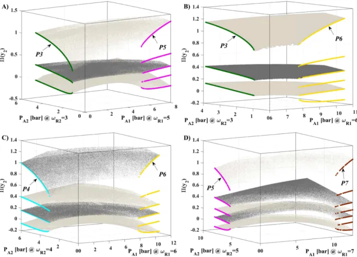
In order to reveal the transformation possibilities between the subharmonic resonances (vertical lines inFig. 3), high-resolution bi-parametric plots are created with the pressure amplitudesP_A1and PA2as control parameters at several fixed relative frequency combinations. According to Eq.(11)and the related discussion, the total number of frequency combinations is 28.Figure 4shows four examples, where the 3D representation of the second component of the Poincaré section is plotted as a function of the control parameters.

The resolutions ofP_A1andP_A2are 801 and 501, respectively. Their ranges are adjusted according to the upper bound of the vertical lines inFig. 3. To find the co-existing attractors, ten randomized initial conditions are applied.

The color-coded branches inFig. 4are periodic orbits using the period of the single-frequency excitationT1 (ifPA2=0) orT2

(ifP_A1=0) for defining a global Poincaré section. The projections of these branches to their control parameter axes inFig. 4 corre- spond to the thick vertical lines in Fig. 3. The arrows mark the period numbers of the solutions. The color-coding is the same as inFigs. 2and3. The dark and light gray points inFig. 4are the period-1 orbits using the period of the dual-frequency drivingTfor defining a global Poincaré section. These solutions form surfaces connecting the colored branches (Fig. 4) in the single-frequency driven limit cases. Therefore, with the proper tuning of the pressure amplitudesPA1 andPA2, the system can be smoothly transformed through the gray surfaces between different periodic orbits of single- frequency driving. It must be stressed that in these figures, three different interpretations are employed for the periodicity according to the definition of the Poincaré section; for the detailed discussion, the reader is referred back to Sec.II C. It is worth noting that the bifurcation structure of the dual-frequency driving is quite complex (see, e.g.,Figs. 2and3in our previous study²³); therefore, only the period-1 orbits are presented inFig. 4to remain focused and avoid overcrowded diagrams.

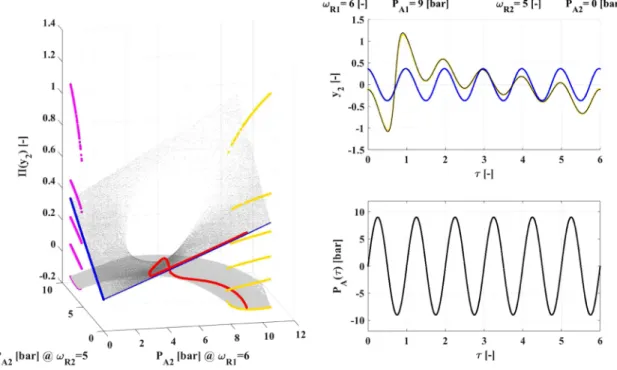
An example of the transformation between a period-4 and a period-6 attractor is demonstrated via an animation that can be found as multimedia. The last frame of the animation is presented inFig. 5(Multimedia view). The 3D panel on the left-hand side of the figure is the second component of the Poincaré section presented already inFig. 4(c). Here, the red curve denotes the route of the transformation. The top panel on the right-hand side shows the dimensionless bubble wall velocityy₂as a function of the dimensionless timeτ. The light blue, yellow, and black curves are the initial (period-4), the final (period-6), and the instantaneous solutions during the transformation, respectively. SinceFig. 5(Multimedia

(7)

FIG. 4. Transformation surfaces between periodic orbits presented by the thick vertical lines inFig. 3via dual-frequency driving. The color-coded branches are periodic orbits of single-frequency driving (sampled withT1orT2), where the labelsP3,. . .,P7 denote their period numbers. The dark and light gray points are period-1 attractors of the dual-frequency driving (sampled withT). Subpanels (a), (b), (c), and (d) are related to the frequency combinations of(ωR1,ωR2)=(5, 3),(6, 3),(6, 4), and(7, 5), respectively.

view) is the last frame of the animation, the yellow and black curves coincide. The bottom panel on the right-hand side is the signal of the external drivingPA(τ )(used here as a general notation for both single- and dual-frequency driving). The thin curve is related to the initial single-frequency driving (ωR2=4, period-4 orbit), while the thick curve is the instantaneous driving signal of the dual- frequency transformation that also ends in a single-frequency driven case (ω_R1=6, period-6 orbit). The values of the control parameters of the external drivingPA1,ω_R1,PA2, andω_R2are depicted as bold texts in the top of the figure/animation. Note that only the pressure amplitudes change during the process. They are updated at every period of the dual-frequency drivingT=6. The rate of change of the amplitudes has to be sufficiently small to remain within the basin of attraction of the solutions.

Although only four examples are shown in Fig. 4, smooth transformations are possible between any pair of periodic orbits.

Keep in mind that the frequency ratio must be equal to the ratio

of the periods (or period numbers) of the orbits being transformed.

For instance, inFig. 4(a), the period numbers are 5 and 3, and the relative frequencies are alsoω_R1=5 andω_R2=3, respectively. Note that not all branches are connected in general. InFig. 4(a), all the green branches are connected to one of the purple branches, while there are purple branches that are not connected to a green branch.

We call this phenomenon partial connectivity. In this sense, the transformation from period-3 to period-5 orbits is “safe,” but the transformation in the opposite direction is “non-safe” (it depends on the initial branch defined by the relative phase in time of the solution). Naturally, there are period-1 surfaces initiated from these

“orphan” branches; however, they are not presented here to avoid overcrowding of the figures. As a final remark, the dual-frequency diagrams can be regarded as connections between one-dimensional bifurcation structures at different frequencies. Compare the two vertical thin lines marked as axis1 and axis2 in Fig. 3 with the dual-frequency case ofFig. 4(d).

(8)

FIG. 5. The last frame of a transformation between a period-4 and a period-6 attractor via a temporary dual-frequency driving, see alsoFig. 4(c). The red curves show the route of the transformation. The top panel on the right-hand side represents the time series of the dimensionless bubble wall velocitiesy2, while the bottom panel on the right-hand side shows the signal of the external drivingPA(τ ). Multimedia view:https://doi.org/10.1063/5.0005424.1

B. Direct routes from period-1 orbits

Another possibility to reach one of the subharmonic periodic domains (period-2 to period-9, vertical lines inFig. 3) is the direct route from period-1 orbits. These period-1 solutions exist below the dashed dark blue codim-2 bifurcation curve shown inFig. 3; see also the dark blue solid line inFig. 2. An example for the direct route is presented inFig. 6produced in the same way as Fig. 4.

The notations, the color-coding, the considerations for the Poincaré sections, and the periodicities are also the same. The employed frequency combination isω_R1=6 andω_R2=5. Here, only a particular period-1 surface (gray) is presented. Its origin is the equilibrium solutiony_2E=0 of the unexcited system; its single-frequency limit cases are depicted by the period-1 (according toT1orT2) blue lines.

Interestingly, the surface tears apart, creating a hole near the middle and extending into an overlapping surface, where one of its sides is connected to a period-5 branch and the other one is attached to a period-6 branch. Panels (a) and (b) ofFig. 6show the same figure from different angles to visualize that the gray points form a single, overlapping surface. This example demonstrates the existence of a direct connection between the period-1 orbits and the subharmonics.

An example of a direct route transformation between a period- 1 and a period-6 attractor is demonstrated via an animation that can be found as multimedia. The last frame of the animation is presented inFig. 7(Multimedia view). The structure of the figure is the same as in the case ofFig. 5(Multimedia view). The 3D panel on the

left-hand side is a copy ofFig. 6in another perspective. The red curve denotes the route of the transformation. Observe that initial and end states of the transformation have the same (single frequency) parameter combination; thus, control of multi-stability is achieved in this specific example. In the top panel on the right-hand side, the blue, yellow, and black curves are the initial (period-1), final (period-6), and instantaneous solutions during the transformation, respectively.

The yellow and black curves coincide sinceFig. 7(Multimedia view) is the last frame of the animation. The bottom panel on the right- hand side is the signal of the external drivingPA(τ ). There is only a single curve here as the initial and end states are related to the same single-frequency driving (ωR1=6). The values of the control parameters of the external drivingPA1,ω_R1,PA2, andω_R2are depicted as bold texts in the top of the figure/animation. Note again that only the pressure amplitudes are changing during the steering process.

Similarly, as in the case of the previous animation, attention has to be paid to the speed of change of the pressure amplitudes.

V. DISCUSSION

Table Isummarizes the possible transformations between periodic attractors of all frequency combinations up to relative frequen- ciesω_R1,2=9. The rows and the columns are related to the high (ωR1) and low (ωR2) relative frequencies, respectively. Due to the normalization via Eqs.(9)and(10), the values ofω_R1 andω_R2are equal to the period numbers of the solutions being transformed.

(9)

FIG. 6. Transformation between period-1 orbits and periodic attractors of the subharmonics. The color-coded branches are periodic orbits of single-frequency driving (sampled withT1orT2), whereP5 andP6 denote their period numbers. The gray points are period-1 attractors of the dual-frequency driving (sampled withT). Panels (a) and (b) show the same figure but from a different perspective to properly visualize the gray surface.

The upper half (due to the symmetry property) and the diagonal (ordinary single-frequency driving) of the table are excluded. The two numbers in each item of the table define the connectivity numbers(c₁,c₂). The first numberc₁describes how many branches are connected from the attractor with the high period number (high frequency,ω_R1) to at least one branch of the solution with the low period number (low frequency,ω_R2). Since the relative frequencies are equal to the period numbers (also the number of the branches) of the solutions being transformed—see the period numbers of the vertical lines inFig. 3and their respective relative frequency values—the transformation fromω_R1toω_R2is “safe” only whenc₁=ω_R1. This condition is fulfilled only in one case discussed below in detail. The second number,c2, describes connectivity in the opposite direction.

Becausec₂=ω_R2in every entry ofTable I, the transformation from a low to a high frequency is always “safe.” That is, all the branches on theω_R2side are connected to at least one branch on theω_R1side.

The label E denotes the transformation possibility directly from the period-1 attractor.

For the majority of the entries inTable I,withoutunderlining, the two connectivity numbers are equal. From these, the bold-faced entries are the cases shown in Sec.IVinFigs. 4and6. Note how the numbers in the table agree with the number of gray surfaces in these figures. As stated before, these cases havepartial connectivity; that is, the transformation is “safe” only in one direction (sincec₁6=ω_R1).

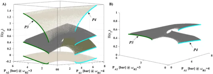
The entrieswithunderlining show frequency pairs having different connectivity numbers (c₁6=c2). Among them, there is only one frequency combination havingfull connectivity:(ω_R1,ω_R2)=(4, 3)

=(c1,c2); see the sole bold-faced entrywithunderlining inTable I.

In this case, all the four branches of the period-4 orbits are connected to one of the branches of the period-3 solutions. This also means that there must be a branch of the period-3 orbits, which is connected to at least two branches of the period-4 attractors. This example is demonstrated inFig. 8(a). It can be seen that there is a surface that is torn apart and connects two branches from the period-4 orbits

to a single branch in its period-3 side. This special surface is also shown in panel (b) from a different perspective for a better view. The other examples inTable Iwithunderlining (but without bold-faced highlighting) have such a property that a single branch on one side is connected to multiple branches on the other side, e.g., frequency combinations(ω_R1,ω_R2)=(5, 2)or(ω_R1,ω_R2)=(8, 5). However, in these cases, the values of the frequency pairs are not equal to the values of the connectivity numbers(ω_R1,ω_R2)6=(c₁,c₂), which means partial connectivity.

In summary, fromTable I, one can conclude that the transformation of the trajectories from low to high periodicity is always

“safe.” That is, regardless of the initial branch on the low period solutions, there always exists a surface that ends on the high period orbits. Observe that the second numbers in the table are always equal to the number in the first row (header line) of the same column. The transformation from high to low periodicity is safe only in the case of the relative frequency combinationω_R1=4 andω_R2=3. Therefore, if one intends to drive the trajectory from a high period solution to a lower one, the pressure amplitude must be tuned down first to reach the period-1 orbit (see, e.g.,Fig. 2), the relative frequency must be adjusted toωR=2, and the pressure amplitude must be tuned up again to be on the period-2 bifurcation branch presented by the red vertical line inFig. 3. From here, the transformation to high periodicities can be initiated that is always safe. Another option is to adjust the system to a period-1 orbit and use one of the direct routes (marked by E inTable I) to reach an orbit with periodicity higher than period 5.

An alternative approach to the presented Attractor Domain Targeting(ADT) method to drive the system to a desired periodic orbit is to set up a proper pair of the pressure amplitude,P_A1, and the relative frequency,ωR1, according toFig. 3. Next, if the system is on an attractor different from the desired one, existing methods²⁴for control of multi-stability can be applied. In order to guarantee that the trajectory shall settle down to the desired orbit, the application

(10)

FIG. 7.The last frame of a transformation (a direct route) between a period-1 and a period-6 attractor via a temporary dual-frequency driving (see alsoFig. 6). The red curve shows the route of the transformation. The top panel on the right-hand side represents the time series of the dimensionless bubble wall velocitiesy2, while the bottom panel on the right-hand side shows the signal of the external drivingPA(τ ). Multimedia view:https://doi.org/10.1063/5.0005424.2

of feedback control^37–50is mandatory. However, there are systems where the application of a feedback control is not possible (as in the case of acoustic bubble models^30,51–61) due to the required continuous sampling of the solution in the state space or even the Jacobian of the system. The ADT technique is a non-feedback method^25,62–81in the sense that no detailed knowledge on the current

TABLE I. Summary of the connectivity numbersc1andc2of the different periodic attractors as a function of the relative frequency combinations. The bold-faced entries without underlining are the cases presented in Sec.IVinFigs. 4and6. The bold-- faced entry with underlining is the sole case withfull connectivityshown inFig. 8. In general, in the case of entries with underlining, the connectivity numbers are not equal (c16=c2).

ω_R₂

2 3 4 5 6 7 8

ω_R1 2 . . . . 3 2, 2 . . . . 4 2, 2 4,3 . . . . 5 3, 2 3, 3 4, 4 . . . . 6 2, 2 3, 3 4, 4 5, 5, E . . . . 7 3, 2 4, 3 4, 4 5, 5 6, 6, E . . . . 8 2, 2 4, 3 4, 4 6, 5 6, 6 7, 7, E . . . 9 4, 2 3, 3 5, 4 6, 5 6, 6 7, 7 8, 8, E

state (and the Jacobian) of the system is required during the transformation. That is, direct attractor selection/targeting is possible—via the transformation surfaces summarized inTable I—without the application of a feedback.This is the main advantage of the ADT method: it enables attractor selection without sampling of the trajec- tory (or the Jacobian) of the solution and without the application of feedback.

The disadvantage of the ADT technique—being a feedforward control method—is that knowledge about the details of the bifurcation structure of the system is required. Otherwise, the proper route of the transformation of the periodic orbits with the temporary dual- frequency driving is not known. The “remedy” for this problem can be the application of an intermediate control quantity, for instance, the spectra of the emitted pressure in the case of bubbles.^82,83The peaks at the subharmonics in the spectra might help to properly tune the driving amplitudes during a transformation. Moreover, if the basin of attraction of the targeted orbit is small, the tuning of the pressure amplitudes PA1 and PA2 must be sufficiently slow. However, the discussion of this issue is beyond the scope of the present study. For a more detailed comparison of the advantages/disadvantages of the proposed ADT technique with methods of control of multi-stability, the interested reader is referred to our previous work.²³

As the ADT method is demonstrated only for a specific system (the Keller–Miksis equation), it is important to generalize the technique to other oscillators/models in the future. As a first step, examining other oscillators such as the Duffing,^84–90Toda,^91–94

(11)

FIG. 8. Example of a frequency combination having branches withfull connectivity. Panel (b) shows the middle surface presented in panel (a) from a different perspective for better visibility.

Morse,^95,96 or van der Pol⁹⁷ equations will be an important step toward the generalization. Furthermore, testing the ADT technique on a large number of diffusively^98–102or globally^103–107coupled iden- tical systems can have great significance as they can exhibit extreme multi-stability¹⁰⁸(the presence of infinitely many co-existing stable states), and they have practical relevance in many scientific areas.

For instance, with the proposed method, it might be possible that in a diffusively coupled model, the rhythmicity can be restored.¹⁰⁹ In acoustic cavitation and sonochemistry,^110–112 the investigation of a bubble cluster^113–116 (an ensemble of single bubbles coupled globally) can provide valuable information on how to drive the system into a chemically highly active state. As a final example, by driving an ultrasound contrast agent into higher-order subharmonics, the resolution of ultrasound imaging can potentially be increased improving the existing techniques in diagnostic ultrasound.^117,118

Finally, it is worth highlighting that any application inherently using dual-frequency excitation for purposes other than controlling multi-stability and attractor targeting can still benefit (at least indi- rectly) from the detailed numerical results presented in this study.

Without giving an exhaustive list, some of these applications are dual-frequency driven sonochemistry,110,119–122stability analysis of traveling beams,^123,124or laser-driven dissociation of molecules.¹²⁵

VI. SUMMARY

A feedforward technique is presented that is capable of driving a periodically driven non-linear system between periodic orbits of subharmonic resonances: theAttractor Domain Targetingtech- nique. This approach is demonstrated with the Keller–Miksis equation describing the evolution of the radial dynamics of a spherical gas bubble placed in an infinite domain of liquid. The basis of the method is the temporary addition of a second harmonic component to the driving. Results have shown that with the proper selection of the frequency pair and with the proper tuning of the amplitudes of the dual-frequency driving, continuous transformations

exist between any pair of periodic orbits of subharmonic resonances.

The technique was numerically tested on attractors with periods up to period 9. The frequency ratio must be equal to the ratio of the periods of the periodic orbits being transformed. As special cases, transformations have been found between period-1 orbits (originating from the equilibrium state of the system in the absence of external forcing) and attractors having a period higher than or equal to 5; see the items marked byEinTable I.

ACKNOWLEDGMENTS

This paper was supported by the Alexander von Humboldt Foundation (Grant No. HUN 1162727 HFST-E), by the János Bolyai Research Scholarship of the Hungarian Academy of Sciences, by the Deutsche Forschungsgemeinschaft (DFG) (Grant No. ME 1645/7- 1), and by the Higher Education Excellence Program of the Ministry of Human Capacities in the frame of Water Science & Disaster Pre- vention research area of the Budapest University of Technology and Economics (No. BME FIKP-VÍZ).

APPENDIX: THE DIMENSIONLESS FORM OF THE KELLER–MIKSIS EQUATION

The Keller–Miksis equation, Eqs.(1)–(4), can be rewritten in a dimensionless form as follows:

˙y1=y2, (A1)

y˙2=N_KM DKM

, (A2)

(12)

where the numerator,NKM, and the denominator,DKM, are NKM= C0+C1y2

1 y1

C10

−C2 1+C9y2

−C3

1 y1

−C4

y2

y1

− 1−C9

y₂ 3

3

2y²₂−(C5sin(2π τ ) +C6sin(2πC₁₁τ+C12)) 1+C9y2

−y₁(C₇cos(2π τ )+C₈cos(2πC₁₁τ+C₁₂)) (A3) and

DKM=y1−C9y1y2+C4C9, (A4) respectively.

The coefficients of the system are summarized as follows:

C₀= 1 ρ_L

P∞−pV+2σ RE

2π REω₁

2

, (A5)

C1=1−3γ ρ_Lc_L

P∞−pV+2σ R_E

2π

R_Eω₁, (A6)

C2=P∞−pV

ρL

2π REω₁

2

, (A7)

C₃= 2σ ρ_LRE

2π REω₁

2

, (A8)

C4= 4µ_L ρ_LR²_E

2π

ω₁, (A9)

C5=P_A1 ρ_L

2π R_Eω₁

2

, (A10)

C₆=PA2

ρL

2π REω1

2

, (A11)

C7=RE

ω₁PA1

ρ_LcL

2π REω₁

2

, (A12)

C8=RE

ω₁P_A2 ρ_Lc_L

2π R_Eω₁

2

, (A13)

C9=R_Eω₁

2πc_L, (A14)

C₁₀=3γ, (A15)

C₁₁=ω₂

ω₁, (A16)

C12=θ. (A17)

DATA AVAILABILITY

The data that support the findings of this study are available from the corresponding author upon reasonable request.

REFERENCES

1J. G. Freire, A. Calderón-Cárdenas, H. Varela, and J. A. C. Gallas, “Phase diagrams and dynamical evolution of the triple-pathway electro-oxidation of formic acid on platinum,”Phys. Chem. Chem. Phys.22, 1078–1091 (2020).

2R. Varga, K. Klapcsik, and F. Heged˝us, “Route to shrimps: Dissipation driven formation of shrimp-shaped domains,”Chaos Soliton Fractals130, 109424 (2020).

3J. A. de Oliveira, L. T. Montero, D. R. da Costa, J. A. Méndez-Bermúdez, R. O. Medrano-T, and E. D. Leonel, “An investigation of the parameter space for a family of dissipative mappings,”Chaos29, 053114 (2019).

4D. W. C. Marcondes, G. F. Comassetto, B. G. Pedro, J. C. C. Vieira, A. Hoff, F. Prebianca, C. Manchein, and H. A. Albuquerque, “Extensive numerical study and circuitry implementation of the Watt governor model,”Int. J. Bifurcat. Chaos 27, 1750175 (2017).

5A. C. C. Horstmann, H. A. Albuquerque, and C. Manchein, “The effect of temperature on generic stable periodic structures in the parameter space of dissipative relativistic standard map,”Eur. Phys. J. B90, 96 (2017).

6R. Rocha and R. O. Medrano-T, “Stability analysis and mapping of multiple dynamics of Chua’s circuit in full four-parameter spaces,”Int. J. Bifurcat. Chaos 25, 1530037 (2015).

7J. A. C. Gallas, “Periodic oscillations of the forced Brusselator,”Mod. Phys. Lett. B 29, 1530018 (2015).

8A. Celestino, C. Manchein, H. A. Albuquerque, and M. W. Beims, “Stable structures in parameter space and optimal ratchet transport,”Commun. Nonlinear Sci.

Numer. Simul.19, 139–149 (2014).

9S. L. T. de Souza, A. A. Lima, I. L. Caldas, R. O. Medrano-T, and Z. O. Guimar˝aes- Filho, “Self-similarities of periodic structures for a discrete model of a two-gene system,”Phys. Lett. A376, 1290–1294 (2012).

10J. G. Freire and J. A. C. Gallas, “Stern–Brocot trees in cascades of mixed- mode oscillations and canards in the extended Bonhoeffer–van der Pol and the Fitzhugh–Nagumo models of excitable systems,”Phys. Lett. A375, 1097–1103 (2011).

11J. G. Freire and J. A. C. Gallas, “Stern-Brocot trees in the periodicity of mixed- mode oscillations,”Phys. Chem. Chem. Phys.13, 12191–12198 (2011).

12A. Celestino, C. Manchein, H. A. Albuquerque, and M. W. Beims, “Ratchet transport and periodic structures in parameter space,”Phys. Rev. Lett.106, 234101 (2011).

13M. A. Nascimento, J. A. C. Gallas, and H. Varela, “Self-organized distribution of periodicity and chaos in an electrochemical oscillator,”Phys. Chem. Chem. Phys.

13, 441–446 (2011).

14S. Luther, F. H. Fenton, B. G. Kornreich, A. Squires, P. Bittihn, D. Hornung, M.

Zabel, J. Flanders, A. Gladuli, L. Campoy, E. M. Cherry, G. Luther, G. Hasenfuss, V. I. Krinsky, A. Pumir, R. F. Gilmour, and E. Bodenschatz, “Low-energy control of electrical turbulence in the heart,”Nature475, 235–239 (2011).

15A. Karma, “Physics of cardiac arrhythmogenesis,”Annu. Rev. Condens. Matter Phys.4, 313–337 (2013).

16J. Tomek, B. Rodriguez, G. Bub, and J. Heijman, “β-Adrenergic receptor stimulation inhibits proarrhythmic alternans in postinfarction border zone car- diomyocytes: A computational analysis,”Am. J. Physiol. Heart Circ. Physiol.313, H338–H353 (2017).

17E. Boccia, S. Luther, and U. Parlitz, “Modelling far field pacing for terminating spiral waves pinned to ischaemic heterogeneities in cardiac tissue,”Philos. Trans.

R. Soc. A375, 20160289 (2017).

18A. E. Motter, S. A. Myers, M. Anghel, and T. Nishikawa, “Spontaneous syn- chrony in power-grid networks,”Nat. Phys.9, 191–197 (2013).

19E. S. Medeiros, R. O. Medrano-T, I. L. Caldas, T. Tél, and U. Feudel,

“State-dependent vulnerability of synchronization,”Phys. Rev. E100, 052201 (2019).

20X. Li, T. Qiu, S. Boccaletti, I. Sendiña-Nadal, Z. Liu, and S. Guan, “Synchro- nization clusters emerge as the result of a global coupling among classical phase oscillators,”New J. Phys.21, 053002 (2019).

21E. S. Medeiros, R. O. Medrano-T, I. L. Caldas, and U. Feudel, “Boundaries of synchronization in oscillator networks,”Phys. Rev. E98, 030201 (2018).

22N. Inaba, H. Ito, K. Shimizu, and H. Hikawa, “Complete mixed-mode oscilla- tion synchronization in weakly coupled nonautonomous Bonhoeffer–van der Pol oscillators,”Prog. Theor. Exp. Phys.2018, 063A01.

(13)

23F. Heged˝us, W. Lauterborn, U. Parlitz, and R. Mettin, “Non-feedback technique to directly control multistability in nonlinear oscillators by dual-frequency driving,”Nonlinear Dyn.94, 273–293 (2018).

24A. N. Pisarchik and U. Feudel, “Control of multistability,”Phys. Rep.540, 167–218 (2014).

25A. N. Pisarchik and B. K. Goswami, “Annihilation of one of the coexisting attractors in a bistable system,”Phys. Rev. Lett.84, 1423–1426 (2000).

26K. Kaneko, “Dominance of Milnor attractors and noise-induced selection in a multiattractor system,”Phys. Rev. Lett.78, 2736–2739 (1997).

27J. B. Keller and M. Miksis, “Bubble oscillations of large amplitude,”J. Acoust.

Soc. Am.68, 628–633 (1980).

28Y. Zhang and Y. Zhang, “Chaotic oscillations of gas bubbles under dual- frequency acoustic excitation,”Ultrason. Sonochem.40, 151–157 (2018).

29H. Haghi, A. J. Sojahrood, and M. C. Kolios, “Collective nonlinear behavior of interacting polydisperse microbubble clusters,”Ultrason. Sonochem.58, 104708 (2019).

30W. Lauterborn and T. Kurz, “Physics of bubble oscillations,”Rep. Prog. Phys.

73, 106501 (2010).

31W. Lauterborn and U. Parlitz, “Methods of chaos physics and their application to acoustics,”J. Acoust. Soc. Am.84, 1975–1993 (1988).

32C. E. Brennen,Cavitation and Bubble Dynamics(Oxford University Press, New York, 1995).

33E. J. Doedel, B. E. Oldeman, A. R. Champneys, F. Dercole, T. F. Fairgrieve, Y. A.

Kuznetsov, R. Paffenroth, B. Sandstede, X. Wang, and C. Zhang,AUTO-07P: Con- tinuation and Bifurcation Software for Ordinary Differential Equations(Concordia University, Montreal, Canada, 2012).

34Seewww.gpuode.comfor “Massively Parallel GPU-ODE Solver (MPGOS)”

(2019).

35F. Heged˝us,MPGOS: GPU Accelerated Integrator for Large Number of Indepen- dent Ordinary Differential Equation Systems(Budapest University of Technology and Economics, Budapest, Hungary, 2019).

36See https://github.com/ferenchegedus/massively-parallel-gpu-ode-solver for

“Massively Parallel GPU-ODE Solver” (2019).

37L. Poon and C. Grebogi, “Controlling complexity,” Phys. Rev. Lett. 75, 4023–4026 (1995).

38U. Feudel and C. Grebogi, “Multistability and the control of complexity,”Chaos 7, 597–604 (1997).

39Y. C. Lai, “Driving trajectories to a desirable attractor by using small control,”

Phys. Lett. A221, 375–383 (1996).

40E. E. N. Macau and C. Grebogi, “Driving trajectories in complex systems,”Phys.

Rev. E59, 4062–4070 (1999).

41S. Gadaleta and G. Dangelmayr, “Learning to control a complex multistable system,”Phys. Rev. E63, 036217 (2001).

42T. Shinbrot, E. Ott, C. Grebogi, and J. A. Yorke, “Using chaos to direct trajectories to targets,”Phys. Rev. Lett.65, 3215–3218 (1990).

43Y. Jiang, “Trajectory selection in multistable systems using periodic drivings,”

Phys. Lett. A264, 22–29 (1999).

44K. Ikeda, “Multiple-valued stationary state and its instability of the transmitted light by a ring cavity system,”Opt. Commun.30, 257–261 (1979).

45K. Ikeda and K. Matsumoto, “High-dimensional chaotic behavior in systems with time-delayed feedback,”Physica D29, 223–235 (1987).

46K. Pyragas, “Continuous control of chaos by self-controlling feedback,”Phys.

Lett. A170, 421–428 (1992).

47B. E. Martínez-Zérega, A. N. Pisarchik, and L. S. Tsimring, “Using periodic modulation to control coexisting attractors induced by delayed feedback,”Phys.

Lett. A318, 102–111 (2003).

48B. E. Martínez-Zérega and A. N. Pisarchik, “Efficiency of the control of coexisting attractors by harmonic modulation applied in different ways,”Phys. Lett. A 340, 212–219 (2005).

49A. N. Pisarchik, R. Meucci, and F. T. Arecchi, “Discrete homoclinic orbits in a laser with feedback,”Phys. Rev. E62, 8823–8825 (2000).

50A. N. Pisarchik, R. Meucci, and F. T. Arecchi, “Theoretical and experimental study of discrete behavior of Shilnikov chaos in a CO2laser,”Eur. Phys. J. D13, 385–391 (2001).

51Y. Zhang, Y. Zhang, and S. Li, “Combination and simultaneous resonances of gas bubbles oscillating in liquids under dual-frequency acoustic excitation,”

Ultrason. Sonochem.35, 431–439 (2017).

52Y. Zhang, Y. Zhang, and S. Li, “The secondary Bjerknes force between two gas bubbles under dual-frequency acoustic excitation,”Ultrason. Sonochem.29, 129–145 (2016).

53A. J. Sojahrood, H. Haghi, Q. Li, T. M. Porter, R. Karshafian, and M. C.

Kolios, “Nonlinear power loss in the oscillations of coated and uncoated bubbles:

Role of thermal, radiation and encapsulating shell damping at various excitation pressures,”Ultrason. Sonochem.66, 105070 (2020).

54A. J. Sojahrood, O. Falou, R. Earl, R. Karshafian, and M. C. Kolios, “Influence of the pressure-dependent resonance frequency on the bifurcation structure and backscattered pressure of ultrasound contrast agents: A numerical investigation,”

Nonlinear Dyn.80, 889–904 (2015).

55K. Yasui, T. Tuziuti, J. Lee, T. Kozuka, A. Towata, and Y. Iida, “The range of ambient radius for an active bubble in sonoluminescence and sonochemical reactions,”J. Chem. Phys.128, 184705 (2008).

56K. Yasui, T. Tuziuti, T. Kozuka, A. Towata, and Y. Iida, “Relationship between the bubble temperature and main oxidant created inside an air bubble under ultrasound,”J. Chem. Phys.127, 154502 (2007).

57K. Yasui, T. Tuziuti, and Y. Iida, “Optimum bubble temperature for the sonochemical production of oxidants,”Ultrasonics42, 579–584 (2004).

58Y. Hao and A. Prosperetti, “The dynamics of vapor bubbles in acoustic pressure fields,”Phys. Fluids11, 2008–2019 (1999).

59L. Stricker and D. Lohse, “Radical production inside an acoustically driven microbubble,”Ultrason. Sonochem.21, 336–345 (2014).

60R. Mettin, I. Akhatov, U. Parlitz, C. D. Ohl, and W. Lauterborn, “Bjerknes forces between small cavitation bubbles in a strong acoustic field,”Phys. Rev. E 56, 2924–2931 (1997).

61R. Mettin, S. Luther, C.-D. Ohl, and W. Lauterborn, “Acoustic cavitation structures and simulations by a particle model,”Ultrason. Sonochem.6, 25–29 (1999).

62E. Li, “Chromatin modification and epigenetic reprogramming in mammalian development,”Nat. Rev. Genet.3, 662–673 (2002).

63V. N. Chizhevsky, “Coexisting attractors in a CO2laser with modulated losses,”

J. Opt. B Quantum Semiclassical Opt.2, 711–717 (2000).

64V. N. Chizhevsky, R. Vilaseca, and R. Corbalán, “Experimental switchings in bistability domains induced by resonant perturbations,”Int. J. Bifurcat. Chaos8, 1777–1782 (1998).

65V. N. Chizhevsky, R. Corbalán, and A. N. Pisarchik, “Attractor splitting induced by resonant perturbations,”Phys. Rev. E56, 1580–1584 (1997).

66V. N. Chizhevsky, E. V. Grigorieva, and S. A. Kashchenko, “Optimal timing for targeting periodic orbits in a loss-driven CO2laser,”Opt. Commun.133, 189–195 (1997).

67V. N. Chizhevsky and P. Glorieux, “Targeting unstable periodic orbits,”Phys.

Rev. E51, R2701–R2704 (1995).

68V. N. Chizhevsky and S. I. Turovets, “Periodically loss-modulated CO2laser as an optical amplitude and phase multitrigger,”Phys. Rev. A50, 1840–1843 (1994).

69K. Kaneko, “Clustering, coding, switching, hierarchical ordering, and control in a network of chaotic elements,”Physica D41, 137–172 (1990).

70V. N. Chizhevsky and S. I. Turovets, “Small signal amplification and classical squeezing near period-doubling bifurcations in a modulated CO2-laser,”Opt.

Commun.102, 175–182 (1993).

71K. Kaneko, “Chaotic but regular posi-nega switch among coded attractors by cluster-size variation,”Phys. Rev. Lett.63, 219–223 (1989).

72B. F. Kuntsevich, A. N. Pisarchik, V. N. Chizhevskii, and V. V. Churakov,

“Amplitude modulation of the radiation of a CO2-laser by optically controlled absorption in semiconductors,”J. Appl. Spectrosc.38, 107–112 (1983).

73L. M. Pecora and T. L. Carroll, “Pseudoperiodic driving: Eliminating multiple domains of attraction using chaos,”Phys. Rev. Lett.67, 945–948 (1991).

74T. L. Carroll and L. M. Pecora, “Using chaos to keep period-multiplied systems in phase,”Phys. Rev. E48, 2426–2436 (1993).

75A. N. Pisarchik, “Controlling the multistability of nonlinear systems with coexisting attractors,”Phys. Rev. E64, 046203 (2001).