Real Estate Price Growth in the World and in Hungary since 1995:

(1)

Real Estate Price Growth in the World and in Hungary since 1995:

Measurement and Explanation

English Language Résumé of the Dissertation

Áron Horváth

Corvinus University of Budapest, Economics Doctoral School February 13, 2008

Abstract

In my dissertation I study the last ten years’developments of the World and of the Hungarian home market. After the survey of the international scienti…c literature in the topic, I analyze the Hungarian residential real estate market. I show that the global house price boom was present in Hungary and the price increase can be explained by the increase of income, the softening credit constraints and the installation of the governmental subsidy system. I complemented the observation of the recent halt of the house price rise with the further rise of the better quality homes. I present a two sector model with better and worse quality homes to describe the latter phenomena.

(2)

1 Introduction

Housing is important not only on its own right, but also as an important fraction of aggregate demand. As real estate wealth constitute an important part of households’

assets, housing prices and rents have an e¤ect on aggregate demand. Housing has become a particularly interesting sector and the topic of many research recently, as prices increased spectacularly since the 1990s in many countries. In my dissertation I …rst present the facts of the global house price boom and survey the literature of the connection between aggregate house prices and macroeconomic variables. At the end of this …rst part I draw the conclusion that it is possible to explain the recent house price boom with macroeconomic factors, i.e. there is no bubble in the house prices, the economic fundamentals are su¢ cient to explain the massive phenomenon. In the second part I reveal the development of the Hungarian house prices. House price index has not been constructed yet in Hungary. Therefore I analyze all the accessible databases and present a calculation which is based on the date collected by me. To catalyze the development of the Hungarian house price index, I surveyed the literature written on the construction methodology of the house price indexes. Moreover I have been cooperating with the experts of the Central Statistical O¢ ce and the National Bank of Hungary. The conclusion of the second part is that the global phenomenon of price movement was observed in Hungary as well, although the indicators measure it with a large margin of error.

The explanation is not obvious, however. The third, last part of my dissertation then gives a possible explanation to this Hungarian phenomena described above.

It is presented in a consistent, structured form of a model. This summary manly focuses on this model.

Macromodels frequently contain a special housing block, where housing demand is treated in the traditional manner: the demand for housing services is determined by the relative price of housing services (rents). Rents and housing prices are related through an asset pricing relationship. The housing stock evolves like the stock of

(4)

capital, and new houses are produced like any other output in a possibly imperfectly competitive market. Thus there are four equations: a supply function (or cost function) and an accumulation identity (a technology condition) characterize the supply side, while the demand side is given by a (conditional) demand function, as well as a an asset pricing equation. These equations determine the four variables of interest: investment in housing, stock of houses, rents and house prices. An important question both theoretically and empirically whether this framework is capable of accounting for the development of the housing market in the last 10 to 15 years. Or, do we need to replace or supplement this framework by adding features like capital market imperfections (e.g credit constraints), market frictions (e.g. costly search), or possibly some bounded rationality behavior as behavioral economists have suggested?

In the following résumé I concentrate on the Hungarian housing market though I hope that the analysis may shed light on the more general question of how to integrate the housing market into a more general macro model. In fact the original purpose of this research was to account for some curious facts pertaining to the Hungarian housing market. In order to accomplish this task, …rst I describe these facts in some detail, identify some salient large shocks that must have a¤ected the housing market, and address the question whether the economy’s actual response to these shocks can be explained by the traditional model. I …nd that one can go a long way to …nd explanations in this manner, but there were some abrupt changes that cannot be squared with the traditional model. One key novel feature of the theoretical framework is vertical di¤erentiation in the housing market, an important feature we deduced from the evolution price data. Though it isn’t proved, there is some reason to believe that this may explain house price developments in Hungary.

(5)

2 Stylized facts and literature review

2.1 International developments

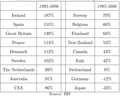
Table 1 shows the cumulated increase in real house prices in 18 developed OECD economies.

Table 1: cumulated increase of real house prices

1995-2006 1995-2006

Ireland 187% Norway 70%

Spain 155% Belgium 60%

Great Britain 139% Finnland 60%

France 114% New-Zealand 53%

Denmark 112% Canada 43%

Sweden 102% Italy 42%

The Netherlands 99% Switzerland 0%

Australia 91% Germany -12%

USA 86% Japan -33%

Source: BIS

The rise is spectacular and almost universal (for details see for example:Girouard et al. [2006] or Himmelberg et al. [2005]) Notice the exceptions: Germany and Japan, and Switzerland to some extent. Germany’s being an outlier is attributed to the construction boom in East Germany after uni…cation, and the consecutive excess supply (seeMilleker [2006]). Japan has its own peculiar economic history in the last two decades, where real estate prices loom both high and low.

Terrones [2004] of the IMF remark that the recent developments are atypical, both the size and the persistence of the price increase are quite exceptional by his- torical standards. They draw attention to the curious fact that house price changes seem to be synchronized internationally, despite houses being usually considered as non-tradables. The price-to-income and the price-to-rent ratios are well above

(6)

their long run trend in almost all countries (Helbling [2005]). It is also remarkable that the price rise was not interrupted by the slowdown of the early 2000s, and the formerly observed procyclicality of house prices may have disappeared.

The phenomenon naturally invited explanations, both standard (Tsatsaronis - Zhu [2004]) and some non-standard (Shiller [2005]) have come along. Standard explanations invoke both demand and supply side factors. With respect to demand there is a claim of higher relative demand for (more and of higher quality housing) due to higher income, and in some cases demographic factors have been enlisted, too. Financial liberalization and the progress of the …nancial infrastructure may have contributed to an increase in demand via alleviating credit constraints, and by making housing investment less expensive.

A number of supply side factors were uncovered, too. It has been pointed out that the construction sector might have had a slower TFP growth than the rest of industry, thereby the real marginal cost of building has gone up. Others have noticed that land prices have constituted an increasing share of housing costs, and this may have been caused by the e¤ective scarcity of land (Glaeser et al. [2005]).

(”E¤ective”, because regulation played a role alongaside geography.) This explanation may be circular, however, since land prices should not be independent of house prices. Still it points to the possibility that construction must have faced increasing marginal costs for technological reasons. Alternatively this may be at variance with an explanation based on higher costs of construction.

(7)

3 Real estate price index construction in Hungary

In a signi…cant part of my research I concentrated on the facts of the Hungarian real estate prices, because there is no house price index in Hungary. First, I surveyed the methodology of creating a house-price index. Simple statistics, repeated sales, hedonic price, hybrid indexes and sales appraisal ratios are studied. The methods are presented with British and U.S. examples. To foster the development of Hungarian house-price indexes, detailed comparison of the various indexes is given. It seems that there is not much digression in the long run trends of the di¤erent indexes, however the di¤erence is signi…cant in the short run. This general statement is demonstrated on a Hungarian database collected from advertisements. In sum, to develop house price indexes one must collect a careful and detailed database in the

…rst place. More than one indexes, based on di¤erent methodologies, are to be constructed and published. Second, I processed the available Hungarian real estate price data bases. Transaction prices of the used homes are collected by the authority and passed to the Central Statistical O¢ ce. I examined this data with the help of the experts of the CSO. Unfortunatelly it found to be very noisy and erronous in many cases, still I calculated some simple statistics from the data. However my results are quite di¤erent from the calculation of the National Bank of Hungary, where a rough …lter is applied on the primer data. To sum up, I demonstrated the Hungarian real estate price rise from three di¤erent data sources but there are large di¤erences with respect to the price changes. As a consequence of the quality of the Hungarian data it is impossible to create an exact house price index as yet, but further work is to be carried out with the experts of the Central Statistical O¢ ce.

Henceforth I treat the Hungarian data as a hard fact, because in the dissertation I mainly focus on qualitative changes.

(8)

3.1 Hungarian developments

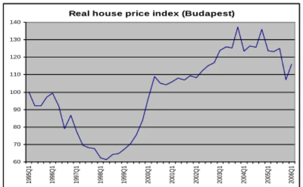
Developments in the Hungarian housing market are quite similar to those discovered above. The notable exception is that the period 1995-2006 divides into two subpe- riods: with a dramatic fall in prices in the …rst and shorter (1995-98) subperiod and an even more spectacular rise in the second (1998-2006). The overall in-sample real price rise amounts to 30%, but is as large as 78% for the period 1998-2004 (see Figure 1).

Figure 1: Real house price index (Budapest)

Real house price index (Budapest)

60 70 80 90 100 110 120 130 140

1995Q1 1996Q1 1997Q1 1998Q1 1999Q1 2000Q1 2001Q1 2002Q1 2003Q1 2004Q1 2005Q1 2006Q1

Source: National Bank of Hungary and own calculation

Even though the general pattern is quite similar and quantitatively comparable to the international developments (documented in Table 1), the possible driving forces behind are not. We will identify factors in‡uencing real estate prices later in Secion 5, and discuss in detail the mechanisms they could have worked through. For a short listing, the country-speci…c e¤ects include the shortage of high quality ‡ats in the beginning of the 1990s (as a heritage of the state-controlled construction sector of the communist system), the large-scale portfolio reallocation after the Russian crises, the initial backwardness and the consequent substantial progress in …nancial intermediation, the steady growth in households’ income starting from 1997, and the high frequency of exogenous shocks to the state subsidies system.

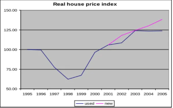
Moreover, a closer look at the Hungarian (Budapest) housing market revealed a new and interesting phenomenon: a widening gap between ’good’and ’bad’quality

(9)

prices for the last couple of years (seeFigure 2).¹

Figure 2: Real house price index (used and new)

Real house price index

50.00 75.00 100.00 125.00 150.00

1995 1996 1997 1998 1999 2000 2001 2002 2003 2004 2005

used new

Source: National Bank of Hungary, Otthon Centrum and own calculation

Part of the gap is attributable to asymmetric subsidies on new and old houses (new constructions were more encouraged by regulation), but change in prerefences could also have played a role. This paper is designed to integrate the speci…c features of the Hungarian housing market into a general model, and provide a coherent and consistent story about the past ten years of the Hungarian housing market.

1I will use ’newly constructed’ and ’old/used’ houses for proxies of ’good’ and ’bad’ quality.

The reason being that houses constructed in the late communist system by all standards inferior to newly built dwellings of the last couple of years.

(10)

4 The model

Aggregate house price modelling was launched by Poterba [1984]. This model is a slight generalization of Topel – Rosen-[1988] as a partial equilibrium model of the housing market with representative agents and a quadratic-linear structure. It contains the traditional features. On the demand side conditional housing demand is derived from a quadratic utility framework. Dynamic utility maximization also implies the asset pricing equation, linking house prices and rents.On the supply side there are cost functions for building new ‡ats, and an accumulation equation. Then pro…t maximization provides the implicit supply functions.

4.1 Households

Representative households (think in terms of extended families living in a modern society) have preferences over houses of higher (HGt), and lower quality (HBt), as well as a numeraire good (Ct). Instantaneous utility is generated according to:

u_t= aHG²_t bHB_t² cHG_t HB_t+ d+d_t HG_t+ (e+e_t)HB_t+f + 1 C_t

All the parameters are non-negative. It is implicitly assumed that housing services are proportional to the stocks of each variety of houses. The relationship a > b is imposed as an expression of vertical (quality) di¤erentiation, positive c represent complemetarity, d_t and e_t are relative preference shocks.

Stocks of the two types of houses develop according to the following processes:

HG_t = (1 _G)HG_t ₁+P G_tDG_t

HB_t = (1 _B)HB_t ₁ +sHG_t ₁+P B_tDB_t

Here DG_t and DB_t denote the purchase of new houses, and P G_t and P B_t their respective prices. The parameter s > 0 means that in each period s percent of

(11)

high quality houses becomes low quality (obsolescence). The parameters represent traditional depreciation.

Household labour and other income (Yt) is exogenous and the intertemporal wealth constraint can be written as:

Y_t+ (1 +r)B_t=B_t+1+C_t+P G_tDG_t+P B_tDB_t;

where r is the constant yield on non-housing investment, = _1+r¹ . Households are unrestricted on capital markets, thus B_t may take on either negative or positive values.

Households maximize an intertemporal utility index

U = X1

t=0

tE_t[u_t]

subject to the above conditions, where <1.

Imposing the transversality condition, and solving the problem of utility maximization yields the following …rst order conditions:

1 =

(where is the marginal utility of income),

( 2aHGt cHBt+ d+dt ) = P Gt

(1 _G)E_t[P G_t+1] +sE_t[P B_t+1] 1 +r

( 2bHB_t cHG_t+ (e+e_t)) = P B_t (1 _B)E_t[P B_t+1] 1 +r :

Rents can be de…ned as:

RG_t = P G_t (1 _G)E_t[P G_t+1] +sE_t[P B_t+1] 1 +r

RB_t = P B_t (1 _B)E_t[P B_t+1] 1 +r :

(12)

Then one can obtain the following static demand functions:

HG_t = 2b d+d_t c(e+e_t) ^2bRG_t+ ^cRB_t 4ab c²

HB_t = 2a(e+e_t) c d+d_t ^2aRB_t+ ^cRG_t 4ab c²

4.2 Construction industry

The representaive building company maximize expected discounted pro…ts. .

= X1

t=0

1 (1 +r)^tE_t

8>

>>

><

>>

:

[P Gt+1; P Bt+1] 2 64 CG_t

CB_t 3 75

K(CG_t; CG_t CG_t ₁; CB_t; CB_t CB_t ₁) 9>

>>

>=

>>

;

We assume that periodtproduction involves costsK(CG_t; CG_t CG_t ₁; CB_t; CB_t CB_t ₁)depending on current production, and also on the adjustment of production with respect to the previous period. (There are convex adjustment costs.) Moreover, there is one period delay between production and selling. Hence …rms must advance funds, whose remuneration is uncertain at the time of expensing. The cost function is quadratic.

K(CG_t; CG_t CG_t ₁; CB_t; CB_t CB_t ₁)

= g₁CG_t+ g₂

2 (CG_t CG_t ₁)²+b₁CB_t+b₂

2 (CB_t CB_t ₁)²

where all parameters are non-negative. The only restriction about the cost function - apart from all parameters being positive - is that high quality houses are more expensive to build than low quality houses, thusg₁ > b₁:

(13)

The implicit supply functions are easily derived from the …rst-order conditions:

g₁+g₂(CG_t CG_t ₁) = 1

1 +rE_t[P G_t+1] b₁ +b₂(CB_t CB_t ₁) = 1

1 +rE_t[P B_t+1]

4.3 Equilibrium

There are two simple equilibrium conditions, according to which houses built in periodt 1 are sold to households in period t.

DG_t = CG_t ₁ DB_t = CB_t ₁:

4.4 The dynamic system

The equations of the linear dynamic system can be summarized as follows:

E_t[P G_t+1]

1 +r = g₁+g₂(CG_t CG_t ₁) E_t[P B_t+1]

1 +r = b1+b2(CBt CBt 1) HG_t = (1 _G)HG_t ₁+CG_t ₁

HB_t = (1 _B)HB_t ₁+sHG_t ₁+CB_t ₁ ( 2aHGt cHBt+ d+dt ) = P Gt

(1 _G)E_t[P G_t+1] +sE_t[P B_t+1] 1 +r

( 2bHB_t cHG_t+ (e+e_t)) = P B_t (1 _B)E_t[P B_t+1] 1 +r

The endogenous variables include:HG_t; CG_t; P G_t; HB_t; CB_t; P B_t:

Our model di¤ers from the Rosen-Topel framework in the following features:

- the housing market exhibits vertical di¤erentiation, - the quality of houses may deteriorate,

- there is a one-period lag between production and selling new houses.

(14)

4.5 The deterministic steady state

In the steady state house prices are determined by marginal costs and the rate of interest, thus are independent of demand. High quality houses are more expensive since they are more costly to build.

P G

1 +r = g1 )P G=g1(1 +r) P B

1 +r = b₁ )P B =b₁(1 +r)

From this, it follows immediately that rents, too, depend on technological parameters and the interest rate.

RG = P G (1 _G)P G+sP B

1 +r = (r+ _G)P G 1 +r

sP B 1 +r RB = P B (1 _B)P B

1 +r = (r+ _B)P G 1 +r

The steady state stocks and new construction can be easily calculated from the demand functions:

HG = 2bd ^2bRG 4ab c² HB = 2ae ^2aRB

4ab c²

HG = (1 _G)HG+CG)CG= _GHG

HB = (1 _B)HB+sHG+CB )CB = _BHB sHG

4.6 Dynamics

While the steady state can be recursively calculated, the solution and analysis of the full dynamic system requires a numerical algorithm. We employed theBlanchard – Kahn [1980] method. To transform our model into this framework we need auxiliary

(15)

variables (Et[P G_t+1]; E_t[P G_t+1]; _t):

P G_t = E_t ₁[P G_t] + ^{P G}_t P B_t = E_t ₁[P B_t] + ^{P B}_t

d_t = _dd_t ₁+"^d_t e_t = _ee_t ₁+"^d_t

The endogenousy_t vector in our case:

y_t= 2 66 66 66 66 66 66 66 66 66 66 66 66 66 64

E_t[P G_t+1] Et[P Bt+1]

P G_t P B_t CG_t CB_t HG_t HB_t d_t e_t

3 77 77 77 77 77 77 77 77 77 77 77 77 77 75

(16)

The coe¢ cient matrices:

0= 2 66 66 66 66 66 66 66 66 66 66 66 66 66 64

1

1+r 0 0 0 g₂ 0 0 0 0 0

0 _1+r¹ 0 0 0 b₂ 0 0 0 0

0 0 0 0 0 0 1 0 0 0

0 0 0 0 0 0 0 1 0 0

1 G

1+r s

1+r 1 0 0 0 2a c 0

0 ¹_1+r^B 0 1 0 0 c 2b 0

0 0 1 0 0 0 0 0 0 0

0 0 0 1 0 0 0 0 0 0

0 0 0 0 0 0 0 0 1 0

0 0 0 0 0 0 0 0 0 1

3 77 77 77 77 77 77 77 77 77 77 77 77 77 75

1 = 2 66 66 66 66 66 66 66 66 66 66 66 66 66 64

0 0 0 0 g₂ 0 0 0 0 0

0 0 0 0 0 b₂ 0 0 0 0

0 0 0 0 1 0 1 _G 0 0 0

0 0 0 0 0 1 s 1 B 0 0

0 0 0 0 0 0 0 0 0 0

1 0 0 0 0 0 0 0 0 0

0 1 0 0 0 0 0 0 0 0

0 0 0 0 0 0 0 0 _d 0

0 0 0 0 0 0 0 0 0 _e

3 77 77 77 77 77 77 77 77 77 77 77 77 77 75

(17)

C = 2 66 66 66 66 66 66 66 66 66 66 66 66 66 64

g₁ b₁ 0 0

d e 0 0 0 0

3 77 77 77 77 77 77 77 77 77 77 77 77 77 75

= 2 66 66 66 66 66 66 66 66 66 66 66 66 66 64

0 0 0 0 0 0 0 0 1 1

3 77 77 77 77 77 77 77 77 77 77 77 77 77 75

= 2 66 66 66 66 66 66 66 66 66 66 66 66 66 64

0 0 0 0 0 0 0 0 0 0 0 0 1 0 0 1 0 0 0 0

3 77 77 77 77 77 77 77 77 77 77 77 77 77 75

We set the baseline parameters to the following values. The interest (discount) rate r = 0:05. Depreciation rates are G = 0;1; _B = 0;1, and s = _G means that good quality homes become bad quality homes after deterioration. By de…nition, good quality homes must be more expensive to construct: g₁ = 200 > b₁ = 150.

We set the adjustment costs to the same in the two sectors:g₂; b₂ = 15. The other parameters have mostly scaling role: d = 50, e = 75, a = 0:5; b = 0:5, c = 0 (we omit the possibility of complementarity), = 2. Finally the setting of the exogenous shock process parameters: z1; z2 = 0:5, _d= 0:9, _e = 0:95.

(18)

5 Shock identi…cation in the Hungarian market

In this section we anecdotically identify shocks in the Hungarian housing market and replicate the e¤ect of these in the model. Our identi…cation process is very rough at this stage of the research: we call an exogenous change a shock in Hungarian housing market, if we think it must have had a signi…cant e¤ect on the housing market. For this ”identi…cation process”we go on step by step through the relevant explanatory variables of the Hungarian housing market.

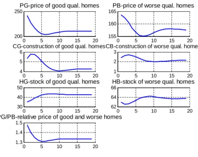
5.1 Quality shortage in the early 1990s

Housing construction was coordinated by central planning during the socialist regime in Hungary. Equality was (is) one of the socialist principles, so houses were mainly built in equal quality. The main memento of this are the numerous blocks of ‡ats all over the country. Therefore, after the regime change a slight shortage of good quality homes was a massive phenomenon in the Hungarian house market (Heged½us – Tosics [1990]). This quality shortage could be easily identi…ed in our model.

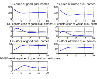
Figure 3 shows the consequences of 20% less stock of good quality homes compared to its long run steady state quantity.

Figure 3: Impulse responses to quality de…cit

0 5 10 15 20

200 250

PG-price of good qual. homes

0 5 10 15 20

155 160 165

PB-price of worse qual. homes

0 5 10 15 20

4 5 6

CG-construction of good qual. homes

0 5 10 15 20

1 2 3

CB-construction of worse qual. homes

0 5 10 15 20

30 40 50

HG-stock of good qual. homes

0 5 10 15 20

62 64 66

HB-stock of worse qual. homes

0 5 10 15 20

1.3 1.4 1.5

PG/PB-relative price of good and worse homes

(19)

If there are less good quality homes, then the relative demand increases their price, so the relative price of good quality homes increases, then slowly moves toward the long run equilibrium. The construction of better quality homes jumps to a relatively high level and then gradually decreases.

5.2 Income growth

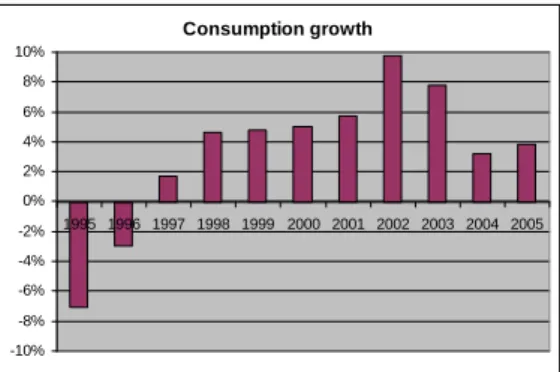
Figure 4a shows the massive income growth Hungary experienced since the end of ninetees. The growth rate of consumption is on Figure 4b. The two patterns look more or less the same, decreasing in 1995 and 1996 and growing permanently afterwards. (There is small di¤erence between the path of income and consumption in the past years, consumption growth was extremely high in 2002 and 2003, and then it slowed to lower pace compared to the income growth.) We identify the robust and steady growth in the real income and consumption since 1997-98 a permanent income shock with our simple identi…cation method.

Figure 4a: Real income per capita growth Figure 4b: Real consumption growth

Real income per capita growth

-10%

-8%

-6%

-4%

-2%

0%

2%

4%

6%

8%

10%

1995 1996 1997 1998 1999 2000 2001 2002 2003 2004 2005

Source: Central Statistical O¢ ce (Hungary)

Consumption growth

-10%

-8%

-6%

-4%

-2%

0%

2%

4%

6%

8%

10%

1995 1996 1997 1998 1999 2000 2001 2002 2003 2004 2005

Source: Central Statistical O¢ ce (Hungary)

In the model income shocks can be identi…ed as the change in parameter , which shows the reciprocal of other goods consumption’s marginal utility. Since our model is calibrated with a constant steady state in the long run, permanent

(20)

growth is omitted at this stage of the analysis. Therefore we formulate the increase of income growth rate with a one time permanent decrease in the marginal utility of consumption, i.e. an increase of . The impulse responses to income’s increase (a one time increase from 0.5 to 3) are shown in Figure 5.

Figure 5: Impulse responses to consumption growth

0 5 10 15 20

0 200 400

0 5 10 15 20

0 200 400

0 5 10 15 20

0 5 10

0 5 10 15 20

0 10 20

0 5 10 15 20

0 50

0 5 10 15 20

0 50 100

0 5 10 15 20

1 1.5 2

The e¤ect of the income growth on prices in the model is an immediate growth of both type of houses’ price, because the relative shortage prevailing at the time of the massive positive demand e¤ect. The construction rapidly increases and then slows to the steady state level, when the quantity of both type of houses are higher.

The relative price of the di¤erent type of houses follows an overshooting path. The relative price of the better houses reaches a higher level than in the steady state.

5.3 The e¤ect of the Russian crisis

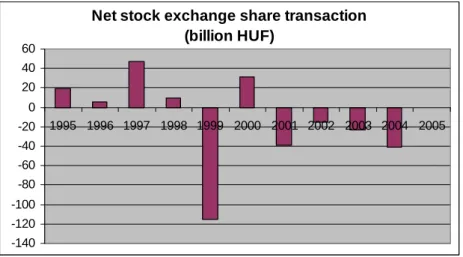
Figure 6 shows a circumstancial evidence of the change in Hungarian investors decision in portfolio investments. There was a signi…cant one time reallocation of portfolios at the expense of shares. There is no evidence that this private portfolio wealth was transposed to real estate wealth only, but together with anecdotical

(21)

evidence from our experience in the late ninetees, it can be identi…ed as a one time permanent demand shock at the housing market.

Figure 6: Portfolio reallocation after the Russian crises

Net stock exchange share transaction (billion HUF)

-140 -120 -100 -80 -60 -40 -20 0 20 40 60

1995 1996 1997 1998 1999 2000 2001 2002 2003 2004 2005

Source: National Bank of Hungary

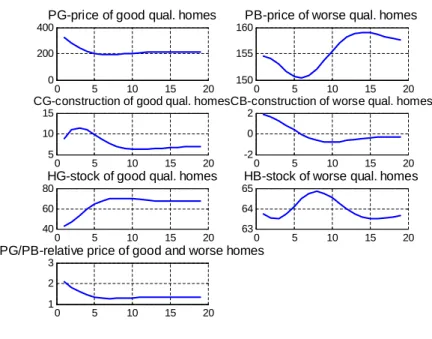
We identify this demand shock in the model with a permanent, additive growth of the demand for housing. However it is less plausible to identify which demand parameter should be changed. We can’t prove our hypothesis, but to the best of our recollection investors portfolio reallocation towards the real estate investments was mainly for better quality houses. So – more or less arbitrarily – we chose to identify the Russian crisis with a one time permament increase in the demand for better quality homes. The impulse responses of this shock (a one time d_t increase ) are shown inFigure 7. The result of the demand growth for better quality houses in the model is an immediate price increase of the better quality homes, and the increase of relative price too. These price variables slowly move back to their long run level, which is determined by the supply side of the model.

(22)

Figure 7: Impulse responses to a permanent demand shock

0 5 10 15 20

0 200 400

0 5 10 15 20

150 155 160

0 5 10 15 20

5 10 15

0 5 10 15 20

-2 0 2

0 5 10 15 20

40 60 80

0 5 10 15 20

63 64 65

0 5 10 15 20

1 2 3

5.4 Financial infrastructure development

The Hungarian …nancial infrastructure started to develop in the mid ninetees. Bank lending was one of the main …eld of the development, and together with the evolution of the legal background mortgage credits became available (Heged½us - Várhegyi [2000]). Figure 8 shows the change of housing loans from the almost zero level.

There was a signi…cant second phase of this process too, when foreign currency loans became available.

Figure 8: Increase of housing loans

Change in housing loans (billion HUF)

-200 0 200 400 600 800

2000 2001 2002 2003 2004 2005 2006

HUF

foreign currency

Source: National Bank of Hungary

(23)

We don’t integrate credit constraints to our simple model, so we identify this development with the decrease of the interest rate. The impulse responses are shown onFigure 9.

Figure 9: Impulse responses to a decrease of the interest rate

0 5 10 15 20

150 200 250

0 5 10 15 20

140 160 180

0 5 10 15 20

2 3 4

0 5 10 15 20

1 2 3

0 5 10 15 20

35 40 45

0 5 10 15 20

55 60 65

0 5 10 15 20

1.32 1.34 1.36

A one time decrease in the interest rate results in an increasing demand for both type of ‡ats. Because of this, prices of both type of ‡ats increase.

5.5 Governmental subsidy system

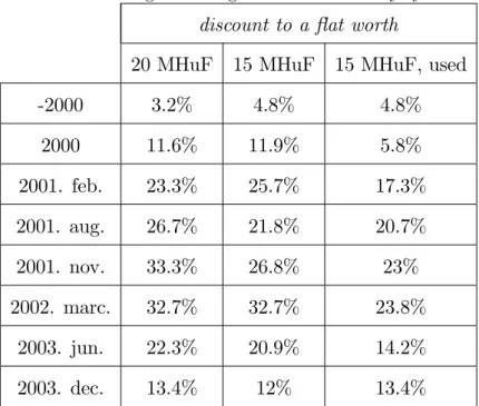
There was a major governmental in‡uence on the Hungarian house market in the last ten years. The government stated a system of subsidies from 2000, which grew in size more and more until it became unsustainable, and was cut to a lower level. The subsidy system contains about 7 policy elements (building allowance, tax refund, mortgage interest subsidy, complementary interest subsidy, redemption subsidy, home saving subsidy, duty subsidy), so it is hard to compress it into few numbers and it is hard to …t into our model. Our rough computation to transform this nontransparent system into our model is made in the following way. We summarized all the possible subsidies to various ‡ats and tried to reconstruct the changes during the last few years. We used past yield curves to calculate the past values of

(24)

interest rate subsidies. Then we summed up the total amount of di¤erent subsidies to a given ‡at. We turned the absolute values into percentage measure. It shows that how much less is paid by the buyer than the selling price is (seeTable 2).

Table 2: Changes in the governmental subsidy system discount to a ‡at worth

20 MHuF 15 MHuF 15 MHuF, used

-2000 3.2% 4.8% 4.8%

2000 11.6% 11.9% 5.8%

2001. feb. 23.3% 25.7% 17.3%

2001. aug. 26.7% 21.8% 20.7%

2001. nov. 33.3% 26.8% 23%

2002. marc. 32.7% 32.7% 23.8%

2003. jun. 22.3% 20.9% 14.2%

2003. dec. 13.4% 12% 13.4%

Source: own calculations based on law.

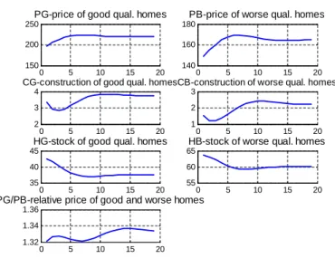
We simulated the e¤ect of a 20% discount in the model.

Figure 10: Impulse responses to permanent governmental subsidy

0 5 10 15 20

200 220 240

0 5 10 15 20

156 157 158

0 5 10 15 20

4 5 6

0 5 10 15 20

1.5 2 2.5

0 5 10 15 20

42 44 46

0 5 10 15 20

63.6 63.8 64

0 5 10 15 20

1.3 1.4 1.5

The e¤ect of subsidies can be easily followed on the above Figure (Figure 11).

Because buyers only pay a discount price, the demand for better quality houses

(25)

increases, and the relative demand is also increase, because better quality homes are subsidized more. Therefore the absolute price, the relative price and the quantity of the better quality homes constructed increase too.

5.6 Confronting the data with the model

We continue with the comparison of the model simulation and the empirical graphs.

Our question is which phenomenon from the past ten years of the Budapest (Hun- garian) residential home market can be explained in the context of our model.

Figure ... showed the graph of used home’s price in Budapest, which we identify as the price of weaker quality homes. There was a signi…cant price increase in Hungary from 1998, and then in 2004 it stopped. After that the relative price of better quality homes rose as shown in Figure... . Construction of new homes in the region is shown on the next …gure (Figure .) New homes are built in signi…cantly better quality than the used ones.

Figure 11: New home construction

new home construction

5 000 7 500 10 000 12 500 15 000 17 500 20 000

1995 1996 1997 1998 1999 2000 2001 2002 2003 2004 2005 Central-Hungary

Central Statistical O¢ ce (Hungary)

The revealed anecdotical empricics are confronted with the model in the next table (Table 3).

(26)

Table 3: Empirics and model simulation results

time and type of the shock model empirics

1995 jumping and decreasing

prices

decreasing price

quality shortage jumping and decreasing relative price

increasing construction of better homes

stagnating construction

1998 jump of both prices

permanent income growth

increasing relativ price fast increase of prices

increasing construction of both type

1998 jumping house prices stagnating construction

Russian crisis jumping and decreasing relative price

increasing construction of better homes

2001 increasing price of better

homes

slowing price increase

governmental subsidy system

signi…cant relative price increase

relative price increase

installed increasing construction of better homes

construction boom

(27)

Table 3 (cont.): Empirics and model simulation results

2001 jumping house prices slowing price increase

softening credit constraints

slowly increasing relative price

relative price increase

increasing construction construction boom increasing price of better

homes

increasing price of better homes

2004 decreasing price of worse

homes

decreasing price of worse homes

subsidy system cutback increasing relative price increasing relative price slowing construction slowing construction To sum up the Table we say that the model can reproduce the overall massive aggregate price increase in the Hungarian home market. The growing income, the portfolio adjustment of the investors after the Russian crisis, the developping …nancial infrastructure and the governmental subsidy system all played a signi…cant role in this process. The model also can reproduce the innovative phenomena in our analysis, the di¤erence between the better and the worse quality homes. Great ma- jority of the new home construction is good, and that’s a corollary of the inherited quality shortage and the character of the governmental subsidy system. The increasing relative price of better quality homes can be explained by the increasing income.

However the time of the consumption boom is unexplained by the model because it started two years later after the demand boom. The empirical observations must be developped in further work.

(28)

6 Summary

In this résumé of my dissertation I concentrated on the Hungarian part of my research. After a short summary of the international literature of the topic I continued to present results I achieved during the analysis. In a short, but important section I presented my attempts to measure the increase of the Hungarian real estate price level. Then as a theoretical achievement I presented a generic model of the housing sector that could easily be integrated into a more general macroeconomic model.

Finally, I tried to replicate some important recent empirical developments of the Hungarian housing market. The novel feature of my contribution (introduction of vertical di¤erentiation into the housing market) is important and provides interesting new insights. While I believe to have done reasonably well in some respects, for a more accurate account of the empirical evidence some speci…c factors and, possibly, some non-standard explanations seem inevitable. Further research should aim at elaborating on these issues.

(29)

References

Blanchard, Olivier J. – Charles Milton Kahn [1980]: The Solution of Linear Di¤erence Models under Rational Expectations. Econometrica, Vol. 48. No. 5.

(July) pp. 1305-1311.

Girouard, Nathalie – Mike Kennedy – Paul van den Noord – Christphe André [2006]: Rescent House price Developments: The Role of Fundamentals. OECD Economics Department Working Paper No. 475.

Glaeser, Edward –Joseph Gyourko –Raven Saks [2005]: Why Have House Prices Gone Up? American Economic Review, Vol. 95. no. 2 (May): pp. 329-333.

Hegedüs József –Tosics Iván [1990]: Hungarian Housing Finance, 1983-1990. A failure of housing reform. Housing Finance International, August, 1990.

Hegedüs József – Várhegyi Éva [2000]: The Crisis in Housing Financing in the 1990’s in Hungary. Urban Studies, Vol. 37, No. 9, pp. 1610-1641.

Helbling, Thomas F. [2005]: Housing Price Bubbles - a Tale Based on Housing Price Booms and Busts. Bank for International Settlements Papers No 21, April 2005.

Himmelberg, Charles –Christopher Mayer –Todd Sinai [2005]: Assessing High House Prices: Bubbles, Fundamentals and Misperceptions. Journal of Economic Perspectives, Vol. 19. no. 4. (Fall 2005): pp. 67-92.

Milleker, David F. [2006]: German residential property: signs of a pick-up in prices. Allianz Dresdner Economic Research Working Paper No 65.

Poterba, James [1984]: Tax Subsidies to Owner-Occupied Housing: An Asset Market Approach. Quarterly Journal of Economics, Vol 99. no. 4.: pp. 729-752.

Terrones, Marco [2004]: What explains the recent run-up in house prices. Box 2.1. In: Terrones - Otrok [2004].

Terrones, Marco –Christopher Otrok [2004]: The Global House Price Boom. In:

IMF World Economic Outlook 2004., pp. 71-89.

(30)

Topel, R – Sherwin Rosen [1988]: Housing Investment in the United States.

Journal of Political Economy, Vol 96. no. 4.: pp. 718-740.

Tsatsaronis, Kostas – Haibin Zhu [2004]: What Drives House Price Dynamics:

Cross-Country Evidence. Bank for International Settlements BIS Quarterly Review, March 2004.

Shiller, Robert [2005]: Long-Term Perspectives on the Current Boom in Home Prices. The Economists’Voice, Vol. 3. no. 4., Article 4.