Calibrating DNN Posterior Probability Estimates of HMM/DNN Models to Improve Social Signal Detection From Audio Data

Calibrating DNN Posterior Probability Estimates of HMM/DNN Models to Improve Social Signal Detection From Audio Data

G´abor Gosztolya

, L´aszl´o T´oth

1

MTA-SZTE Research Group on Artificial Intelligence, Szeged, Hungary

2

University of Szeged, Institute of Informatics, Szeged, Hungary

{ ggabor, tothl } @ inf.u-szeged.hu

Abstract

To detect social signals such as laughter or filler events from audio data, a straightforward choice is to apply a Hidden Markov Model (HMM) in combination with a Deep Neural Net- work (DNN) that supplies the local class posterior estimates (HMM/DNN hybrid model). However, the posterior estimates of the DNN may be suboptimal due to a mismatch between the cost function used during training (e.g. frame-level cross- entropy) and the actual evaluation metric (e.g. segment-level F1 score). In this study, we show experimentally that by em- ploying a simple posterior probability calibration technique on the DNN outputs, the performance of the HMM/DNN work- flow can be significantly improved. Specifically, we apply a linear transformation on the activations of the output layer right before using the softmax function, and fine-tune the parameters of this transformation. Out of the calibration approaches tested, we got the bestF1scores when the posterior calibration process was adjusted so as to maximize the actual HMM-based evalua- tion metric.

Index Terms: social signals, laughter detection, filler events, Hidden Markov Model, Deep Neural Networks, posterior prob- ability calibration

1. Introduction

Non-verbal communication plays an important role in human speech comprehension. Besides specific visual cues, some types of messages can be transferred by non-verbal vocaliza- tions (laughter, filler events, throat clearing, breathing) as well.

The interpretation of speakers’ intentions can be assisted by us- ing paralinguistic information; for instance, to acquire informa- tion about the speaker’s emotional state and attitudes [1], or to recognize equivocation and irony [2]. Detecting specific non- verbal phenomena such as laughter and filler events may also assist automatic speech recognition (ASR) systems and help re- duce the word error rate.

To detect social signals in an audio recording, the simplest approach is to train and evaluate the actual machine learning method at the frame level. But one would expect better re- sults from a solution that works over segments, for which a straightforward choice is to utilize a Hidden Markov Model (HMM), which incorporates some frame-level model – such as a Deep Neural Network (DNN) – that supplies the local (frame- level) posterior probability estimates of the specific acoustic events. This HMM/DNN hybrid technology is now standard in speech recognition [3]. To improve the performance of this HMM/DNN hybrid, it is common to fine-tune several meta- parameters related to DNN structure, to DNN training, or to the HMM part; it is quite rare, however, to applyposterior proba- bility calibrationto the DNN outputs before utilizing them in the HMM.

The main goal of calibration is to turn the output scores of a classifier into valid posterior class probability estimates. No- table examples for this mechanism are the classification rule of AdaBoost.MH [4] and Support-Vector Machines (SVMs, [5]), as the output values of these classifiers cannot be directly in- terpreted as posterior probabilities. Deep Neural Networks, at a first glance, do not fall into this category, as DNN training via the cross-entropy error function was proven to provide not only competitive classification accuracies, but also reliable pos- terior estimates [6]. Yet, in the HMM/DNN hybrid model, there is still a mismatch between trainining the DNN forframe-level classification, while we want to minimize some objective func- tion that is defined at theutterance level, like the Word Error Rate (WER) in the case of speech recognition. To alleviate this gap, sequence-level optimization methods were proposed for HMMs [7, 8], and now these are routinely used for HMM/DNN hybrids as well [9, 10]. Unfortunately, these methods are un- likely to work well in the case of audio event detection, first because we seek to optimize a different metric (e.g. theF1

score), and second because laughter and filler events take up only a fraction of the sequence duration. This class imbalance is known to be problematic for sequence-level training (known as the ‘runaway silence model’ issue [11]).

When training the DNN at the frame level, a number of other factors might also contribute to the posterior estimates to be imprecise to the extent that it leads to a suboptimal HMM/DNN performance. For example, DNNs are known to be biased towards classes having more training examples [12], and in our case, a significant class imbalance is clearly present. An- other possible source of suboptimality might be the imprecise positioning of the DNN training targets. Regardless of whether these frame-level class labels come from a manual annotation or from an automated forced-aligned process, they are prone to noise due to the imprecise positioning of phonetic or social sig- nal occurrence boundaries, and this noise is propagated further to the output of the HMM. Therefore the DNN outputs might need to be adjusted to improve utterance-level performance;

finding this transformation is the posterior calibration process itself. Altogether, these are the reasons why we expect to gain better performance from calibrating the posterior estimates pro- duced by a DNN trained with frame-level targets.

A number of calibration techniques have been developed such as Platt scaling, logistic regression and isotonic regres- sion (see e.g. [5, 13, 14]), and these were used in several scientific areas such as direct marketing analysis [15], med- ical diagnosis [16], psychology [17] and emotion classifica- tion [18]. Furthermore, posterior calibration was employed in HMM-based frameworks in various areas like natural language processing [19] and dynamic travel behavioral analysis [20].

However, we found no study that calibrated the posterior es-

timates of HMM/DNN models using audio as the input. In this study we present our approach of posterior calibration for de- tecting laughter and filler events in spontaneous conversation.

Our approach is a simple-yet-effective DNN-specific method:

we linearly transform the neuron activations in the output layer just before applying the softmax function. By tuning the pa- rameters of this transformation on the development set, we re- port relative error reduction scores of 6-7% on the test set of a public database containing English spontaneous telephone con- versations.

2. Posterior Calibration for HMM/DNNs

A standard Hidden Markov Model requires frame-level esti- mates of the class-conditional likelihoodp(xt|ck)for the obser- vation vectorxtand for each classck, which are traditionally provided by a Gaussian Mixture Model (GMM) [21]. Neural networks, however, are discriminative classifiers (in contrast to GMMs which are generative ones), which means that they esti- mate theP(ck|xt)values. From these estimates, thep(xt|ck) values expected by the HMM can be got using Bayes’ theorem, i.e.:

p(xt|ck) = P(ck|xt)·P(xt)

P(ck) . (1)

So, in a HMM/DNN hybrid, we divide the posterior estimates produced by a DNN by theP(ck)a priori probabilities of the classes. This will give us the required likelihood values within a scaling factor (the combined probability of thextobservation vectors), which can be ignored as it has no influence on the subsequent maximum a posteriori (MAP) decision process.

2.1. Posterior Calibration for Deep Neural Networks In standard DNNs, when utilized for classification, the number of output neurons is set equal to the number of classes, and we employ the softmax activation function in the output layer. This guarantees that the output values are non-negative and add up to one, so they satisfy the formal requirements of a posterior estimate. Formally,

P(ck|xt) =σ(z)j= e^zj PK

k=1e^zk, (2) wherezj are the linear activation values of the corresponding neurons. In the simplest form of posterior calibration, we per- form a linear transformation on thezj values, i.e. we replace them by

z^′_j=ajzj+bj. (3) Notice that we have two tunable parameters (aandb) for each output neuron.

2.2. Optimization

In the above we did not consider the choice of the actual opti- mization method to be an essential part of the proposed work- flow: in the posterior probability calibration approach outlined above we could use practically any algorithm. For example, as the transformation we propose is linear, it could be easily incor- porated into the backpropagation optimization process. How- ever, ideally we would like to optimize the performance of the whole system for sentence-level detection. For this, we would have to define an error function that is differentiable and ex- presses the sentence-level detection errors. Here, we will use an evaluation metric that is derived from the F1 score. Al- though attempts have been made to formalize theF1 error in

backpropagation-based DNN training [22], the results are not convincing. Furthermore, we would like to use a metric defined over segments, not simple frames (see Section 3.2 for details).

For these reasons, we decided to apply general-purpose opti- mization methods.

Since the number of parameters we have to tune is twice the number of classes, even to detect two phenomena (and hav- ing one class for the background) means a six-dimensional op- timization problem. Unfortunately, the straightforward choice of grid search is unfeasible even for a small number of events, so we need more sophisticated methods. In the experimental validation of the proposed workflow, we will test two such op- timization approaches.

The first optimization technique tested was generating random valuesand choosing the vector which leads to the best performance on the development set. Though this may seem to be a primitive technique at first glance, it was shown (see e.g.

the study of Bergstra and Bengio [23]) that this is a favorable method to grid search for hyper-parameter optimization. There- fore we generated randomaandbvectors following a uniform distribution, performed a search with HMM on the development set, and chose the vector which led to the highestF1scores.

The other optimization approach we used is theCovari- ance Matrix Adaptation Evolution Strategy(CMA-ES, [24]) method for meta-parameter optimization. Evolution Strate- gies resemble Genetic Algorithms in that they mimick the evo- lution of biological populations by selection and recombina- tion, so they are able to “evolve” solutions to real world prob- lems. CMA-ES is reported to be a reliable and competitive method for badly conditioned, non-smooth (i.e. noisy) or non- continuous problems [25]. Furthermore, it requires little or no meta-parameter setting for optimal performance. Here, we used the Java implementation with the default settings.

3. Experimental Setup

3.1. The SSPNet Vocalization Corpus

We performed our experiments on the SSPNet Vocalization Corpus [26], which consists of short audio clips from En- glish telephone conversations. The total recording time of this corpus is 8 hours and 25 minutes with 2988 laughter and 1158 filler events. Since in the public annotation only the laughter and filler events are marked, in our experiments we had three classes, namely “laughter” (3.4%), “filler” (4.9%) and “other” (meaning both silence (40.2%) and non-filler non- laughter speech (51.3%)). We used the standard split of the dataset into a training, development and test set, introduced in the ComParE 2013 Challenge [27]. From the total of 2763 clips, 1583 were assigned to the training set, while 500 clips were as- signed to the development set, and 680 clips to the test set.

3.2. Evaluation Metrics

For tasks like social signal detection, where the distribution of classes is significantly biased, classification accuracy is only of limited use. Another common metric used in social signal de- tection is to take the AUC score of the frame-level posteriors as in e.g. [27, 28]. However, in our opinion the performance of a method can be more reliably judged by utilizing a HMM and measuring the quality of event occurrence hypotheses. We opted for the information retrieval metrics ofprecision,recall andF-measure(orF¹), which we regard as straightforward and appropriate metrics for the current task. We summarized the scores of the two social signals bymacro-averaging: we aver-

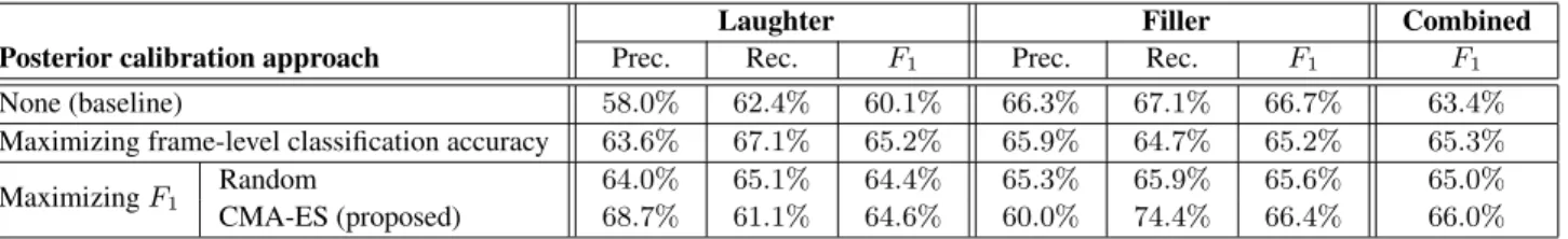
Laughter Filler Combined

Posterior calibration approach Prec. Rec. F1 Prec. Rec. F1 F1

None (baseline) 58.0% 62.4% 60.1% 66.3% 67.1% 66.7% 63.4%

Maximizing frame-level classification accuracy 63.6% 67.1% 65.2% 65.9% 64.7% 65.2% 65.3%

MaximizingF1

Random 64.0% 65.1% 64.4% 65.3% 65.9% 65.6% 65.0%

CMA-ES (proposed) 68.7% 61.1% 64.6% 60.0% 74.4% 66.4% 66.0%

Table 1: Optimalsegment-levelaveraged F-measure values on the test set when using different strategies for posterior calibration.

aged the precision and the recall scores of these two phenom- ena, and calculatedF¹from these average values.

To decide whether a laughter occurrence hypothesis re- turned by the HMM and one labelled by a human annotator match (i.e. segment-level evaluation), we combined two re- quirements. First, we required that the two occurrences refer to the same kind of event (i.e. laughter or filler) and that their time intervals intersected (e.g. [29, 30, 31]). Second, the center of the two occurrences had to be close to each other (i.e. within 500ms). The latter requirement was inspired by the NIST stan- dard for Spoken Term Detection evaluation [32].

As it is also common to calculate precision, recall and F- measure at the frame level, we will also report the effective- ness of the posterior probability calibration techniques when taking these values at the level of frames. Similar to the case of segment-level evaluation, here we again averaged out the preci- sion and the recall scores of the two types of events. Obviously, we optimized theaandbvectors for the two (evaluation) met- rics independently, always optimizing the actual metric.

3.3. DNN Parameters

As the DNN component of our hybrid recognizer, we used our custom implementation, which achieved the lowest error rate on the TIMIT database ever published with a phonetic error rate of 16.5%on the core test set [33]. Following the results of our previous studies (see [34]), we utilized DNNs with five hidden layers, each containing 256 rectified neurons, and applied the softmax function in the output layer.

We used the feature set introduced in the ComParE 2013 Challenge [27], which consists of the frame-wise MFCC +∆+

∆∆feature vector along with voicing probability, HNR,F0and zero-crossing rate, and their derivatives. To these 47 features their mean and standard derivative in a 9-frame neighbourhood were added, resulting in a total of 141 features, extracted with the openSMILE tool [35]. Again, following our previous works, we extended the feature vectors with the features of 16 neigh- bouring frames from both sides, resulting in a 33 frame-wide sliding window [34].

It is known that DNN training is a stochastic procedure due to random weight initialization. To counter this effect, we trained five DNN models in an identical way (except the ran- dom seed value), and averaged out the precision, recall andF1

scores. This was done both for the baseline models and in the experiments using the calibrated posteriors.

3.4. HMM State Transition Probabilities

Our HMM consisted of only three states, each one represent- ing a different acoustic event. In this set-up, the state transition probabilities of the HMM practically correspond to a language model. Following Salamin et al. [26], we constructed a frame- level state bi-gram. The transition probability values were cal-

culated on the training set, and we used the development set to find the optimal language model weight for each (transformed) DNN model independently.

3.5. Calibration Parameter Optimization

Since we calibrated the posterior estimates for three classes, we had a six-dimensional optimization task. In accordance with Section 2, we optimized these parameters on the development set, while the final model evaluation was carried out on the test set. Theaandbvectors were expected to remain in the range [−25,25]. The CMA-ES optimization method allows us to set the vector where the search process is initiated; we made the straightforward choice of using the original posterior estimates for this aim (i.e. we had the starting values ofa= 1andb= 0).

The optimization process was allowed to run for 2000 iterations;

as for the random optimization process, we also generated 2000 vectors overall. We optimized theaandbtransformation pa- rameter vectors for the five DNN models independently.

For comparison, we also tested the approach where we choose the transformation parameters that produce the best frame-level classification of the development set. That is, af- ter re-scaling the frame-level DNN outputs following Bayes’

theorem using the a priori estimates, we choose the class for each frame with the highest transformed likelihood, and calcu- late the traditional classification accuracy relative to the frame- level manual annotation.

4. Results

Table 1 shows the obtainedsegment-levelprecision, recall and F¹ scores on the test set. The baseline scores are around 60- 66%, which is standard on this dataset (see e.g. [31, 34]). Also notice that filler events were identified more precisely (about 66%) than laughter events (58-62%). When performing poste- rior probability calibration by maximizing frame-level classifi- cation accuracy, we obtained an average combined F-measure score of 65.3%; most of this improvement came from more precise laughter detection. Although the improvement is only 1.9% absolute (5% relative), it was found to be significant with p <0.01by the Mann-Whitney-Wilcoxon ranksum test [36]

When incorporating the HMM search step in the calibra- tion process and trying out randomaandbvectors (case “Max- imizingF1– Random”), we managed to improve theF1score for laughter by 4.3% absolute over the baseline score; in terms of relative error reduction (RER), it means an 11% improve- ment. Although the various scores associated with the filler events fell slightly, the average combinedF1 score rose from 63.4% to 65.0%. Unfortunately, this improvement is not signif- icant even withp= 0.05. However, when we maximized the utterance-levelF1 score after using the HMM, and employed the CMA-ES method to find the optimalaandbtransformation

Laughter Filler Combined

Posterior calibration approach Prec. Rec. F1 Prec. Rec. F1 F1

None (baseline) 54.6% 70.4% 61.4% 54.3% 62.6% 58.1% 59.8%

Maximizing classification accuracy 74.7% 50.7% 60.3% 63.2% 53.9% 58.2% 59.4%

MaximizingF1

Random 61.1% 68.2% 64.4% 62.4% 56.4% 59.2% 62.0%

CMA-ES (proposed) 64.9% 66.0% 65.3% 54.0% 65.4% 59.2% 62.4%

Table 2: Optimalframe-levelaveraged F-measure values on the test set when using different strategies for posterior calibration.

Time (sec)

0 1 2 3 4 5 6

Posterior estimates

0 0.2 0.4 0.6 0.8 1

Laughter

Filler

Laughter (original) Filler (original) Laughter (calibrated) Filler (calibrated)

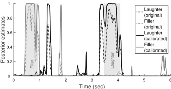
Figure 1:A sample of the original (dotted lines) and calibrated (continuous lines) posterior estimates; the shaded regions indi- cate the annotated occurrences.

vectors (case “MaximizingF1– CMA-ES”), we got a combined segment-level F1 score of 66.0%, meaning a 7% RER score, which was found to be significant withp <0.01.

At theframe level(see Table 2), we notice that optimizing the posterior calibration parameters for classification actually led to a drop in our metric scores. This is especially surpris- ing as the very same values led to a (significant) increase in the segment-level values. This difference is most apparent in the case of the laughter events: while we could improve their de- tection at the segment level, our frame-level values (especially the recall scores) fell dramatically. This is consistent with our previous finding (see e.g. [34]) that, since laughter events are fairly long phenomena (in this corpus their average duration is 942ms), it is relatively easy to finda part of them. Their exact starting and ending points, however, are quite hard to identify.

Indeed, the (frame-level) recall score for laughter events is be- low that of the baseline for all calibration approaches tested.

Due to this drop in theF1score for laughter events, the com- binedF¹ score appeared to be lower as well (since there was practically no change in the filler event detection performance).

Incorporating the HMM search into the posterior proba- bility calibration process, however, led to significant improve- ments (p <0.01) in both cases. For random values, we got an absolute improvement of 2.2% (5% RER), while utilizing the CMA-ES algorithm to set the calibration parameters led to a combinedF1score of 62.4% (7% RER). Most of the improve- ment came from a higher precision score of the laughter events for both approaches; since the corresponding recall scores re- mained at the baseline level, we think that calibration led to less false alarms in the case of laughter events.

Fig. 1 shows a sample from an utterance of the test set.

We can readily see that the original posterior estimates (dot- ted lines) are lower than the calibrated ones (continuous lines).

It is also quite apparent that, although the HMM/DNN model obviously found the two annotated occurrences (the two shad-

owed regions) in this excerpt, the boundaries of the HMM/DNN hypotheses and the manual annotation match only loosely. This difference, in our opinion, demonstrates the amount of subjec- tivity inevitably present in the frame-level annotation of social signals, which is why we consider the segment-level perfor- mance measurement approach both more meaningful and more reliable. Nevertheless, regardless of the use of segment- or frame-level F1 to measure event detection accuracy, the pro- posed posterior probability calibration technique significantly improved the performance of the HMM/DNN hybrid.

5. Conclusions

In this study, we focused on the DNN acoustic models of HMM/DNN hybrids used for social signal detection. To boost the performance, we applied posterior probability calibration;

that is, we applied a linear transformation on the activations of the output layer just before using the softmax function, and fine- tuned the transformation parameters. We experimented with several approaches for finding the optimal values of this linear transformations. Our results indicate that it is indeed benefi- cial to incorporate the search step of Hidden Markov Models into the optimization process, and utilizing the Covariance Ma- trix Adaptation Evolution Strategy (CMA-ES) method led to better results than generating random vectors did. Evaluated on segment-level and on frame-level, the proposed approach in both cases led to significant improvements in the performance.

On examining the original and the calibrated (transformed) posterior estimates, we found that posterior probability calibra- tion markedly increased the probability estimates of the rarer classes (in our case, laughter and filler events). This was not really surprising, as neural networks are known to overesti- mate the probability of more frequent classes and underestimate those which have less training data. Although we divide these posterior estimates by the priors before utilizing them in the HMM, which step increases the relative importance of these mi- nority classes, we found that a further increase was required to achieve optimal performance in terms of frame- and segment- level F-measure scores. Of course, it would be interesting to evaluate the proposed approach in a multi-language set-up. This is, however, clearly the subject of future work.

6. Acknowledgements

This research was partially funded by the National Research, Development and Innovation Office of Hungary via contract NKFIH FK-124413, and by the Ministry of Human Ca- pacities of Hungary (grants 20391-3/2018/FEKUSTRAT and TUDFO/47138-1/2019-ITM). G. Gosztolya and L. T´oth were also funded by the J´anos Bolyai Scholarship of the Hungarian Academy of Sciences, and by the Ministry of Innovation and Technology New National Excellence Program ´UNKP-19-4.

7. References

[1] M. T. Suarez, J. Cu, and M. S. Maria, “Building a multimodal laughter database for emotion recognition,” inProceedings of LREC, 2012, pp. 2347–2350.

[2] F. Burkhardt, B. Weiss, F. Eyben, J. Deng, and B. Schuller, “De- tecting vocal irony,” inProceedings of GSCL, Berlin, Germany, Sep 2017, pp. 11–22.

[3] G. Hinton, L. Deng, D. Yu, G. E. Dahl, A.-r. Mohamed, N. Jaitly, A. Senior, V. Vanhoucke, P. Nguyen, T. N. Sainathet al., “Deep neural networks for acoustic modeling in speech recognition: The shared views of four research groups,”IEEE Signal Processing Magazine, vol. 29, no. 6, pp. 82–97, 2012.

[4] R. E. Schapire and Y. Singer, “Improved boosting algorithms using confidence-rated predictions,”Machine Learning, vol. 37, no. 3, pp. 297–336, 1999.

[5] J. Platt, “Probabilistic outputs for Support Vector Machines and comparison to regularized likelihood methods,” inAdvances in Large Margin Classifiers, A. Smola, P. Bartlett, B. Schoelkopf, and D. Schuurmans, Eds. MIT Press, 2000, pp. 61–74.

[6] H. Bourlard and N. Morgan,Connectionist Speech Recognition – A Hybrid Approach. Kluwer Academic, 1994.

[7] Y. Normandin, R. Lacouture, and R. Cardin, “MMIE training for large vocabulary continuous speech recognition,” inProceedings of ICSLP, Yokohama, Japan, Sep 1994, pp. 1367–1370.

[8] D. Povey and P. C. Woodland, “Improved discriminative training techniques for large vocabulary continuous speech recognition,”

inProceedings of ICASSP, Salt Lake City, UT, USA, May 2001, pp. 45–48.

[9] G. Gosztolya, T. Gr´osz, and L. T ´oth, “GMM-free flat start sequence-discriminative DNN training,” inProceedings of Inter- speech, San Francisco, CA, USA, Sep 2016, pp. 3409–3413.

[10] D. Povey, V. Peddinti, D. Galvez, P. Ghahremani, V. Manohar, X. Na, Y. Wang, and S. Khudanpur, “Purely sequence-trained neu- ral networks for ASR based on lattice-free MMI,” inProceedings of Interspeech, San Francisco, CA, USA, Sep 2016, pp. 2751–

2755.

[11] H. Su, G. Li, D. Yu, and F. Seide, “Error back propagation for sequence training of Context-Dependent Deep Networks for con- versational speech transcription,” inProceedings of ICASSP, Van- couver, Canada, May 2013, pp. 6664–6668.

[12] L. T ´oth and A. Kocsor, “Training HMM/ANN hybrid speech rec- ognizers by probabilistic sampling,” inProceedings of ICANN, 2005, pp. 597–603.

[13] A. Niculescu-Mizil and R. Caruana, “Obtaining calibrated proba- bilities from boosting,” inProceedings of UAI, 2005, pp. 413–420.

[14] G. Gosztolya and R. Busa-Fekete, “Calibrating AdaBoost for phoneme classification,”Soft Computing, vol. 23, no. 1, pp. 115–

128, 2019.

[15] K. Coussement and W. Buckinx, “A probability-mapping algo- rithm for calibrating the posterior probabilities: A direct market- ing application,”European Journal of Operational Research, vol.

214, no. 3, pp. 732–738, 2011.

[16] W. Chen, B. Sahiner, F. Samuelson, A. Pezeshk, and N. Pet- rick, “Calibration of medical diagnostic classifier scores to the probability of disease,”Statistical Methods in Medical Research, vol. 27, no. 5, pp. 1394–1409, 2018.

[17] G. van Kollenburg, J. Mulder, and J. K. Vermunt, “Posterior cali- bration of posterior predictive p values,”Psychological Methods, vol. 22, no. 2, pp. 382–396, 2017.

[18] G. Gosztolya and R. Busa-Fekete, “Posterior calibration for multi- class paralinguistic classification,” inProceedings of SLT, Athens, Greece, Dec 2018, pp. 119–125.

[19] K. Nguyen and B. O’Connor, “Posterior calibration and ex- ploratory analysis for natural language processing models,” in Proceedings of EMNLP, Lisbon, Portugal, Sep 2015, pp. 1587–

1598.

[20] C. Xiong, D. Yang, J. Ma, X. Chen, and L. Zhang, “Measuring and enhancing the transferability of hidden markov models for dynamic travel behavioral analysis,”Transportation, vol. online first, pp. 1–21, 2018.

[21] R. Duda and P. Hart,Pattern Classification and Scene Analysis.

Wiley & Sons, New York, 1973.

[22] F. Milletari, N. Navab, and S.-A. Ahmadi, “V-Net: Fully convo- lutional neural networks for volumetric medical image segmenta- tion,” inProceedings of 3DV, Stanford, CA, USA, Oct 2016, pp.

565–571.

[23] J. Bergstra and Y. Bengio, “Random search for hyper-parameter optimization,” Journal of Machine Learning Research, vol. 13, pp. 281–305, 2012.

[24] N. Hansen and A. Ostermeier, “Completely derandomized self- adaptation in evolution strategies,” Evolutionary Computation, vol. 9, no. 2, pp. 159–195, 2001.

[25] N. Hansen and S. Kern, “Evaluating the CMA evolution strat- egy on multimodal test functions,” inParallel Problem Solving from Nature PPSN VIII, ser. LNCS, X. Yaoet al., Eds., vol. 3242.

Springer, 2004, pp. 282–291.

[26] H. Salamin, A. Polychroniou, and A. Vinciarelli, “Automatic de- tection of laughter and fillers in spontaneous mobile phone con- versations,” inProceedings of SMC, 2013, pp. 4282–4287.

[27] B. Schuller, S. Steidl, A. Batliner, A. Vinciarelli, K. Scherer, F. Ringeval, M. Chetouani, F. Weninger, F. Eyben, E. Marchi, H. Salamin, A. Polychroniou, F. Valente, and S. Kim, “The Inter- speech 2013 Computational Paralinguistics Challenge: Social sig- nals, Conflict, Emotion, Autism,” inProceedings of Interspeech, 2013.

[28] R. Gupta, K. Audhkhasi, S. Lee, and S. S. Narayanan, “Speech paralinguistic event detection using probabilistic time-series smoothing and masking,” inProceedings of InterSpeech, 2013, pp. 173–177.

[29] G. Gosztolya, “On evaluation metrics for social signal detection,”

inProceedings of Interspeech, Dresden, Germany, Sep 2015, pp.

2504–2508.

[30] F. B. Pokorny, R. Peharz, W. Roth, M. Z ¨ohrer, F. Pernkopf, P. B. Marschik, and B. Schuller, “Manual versus automated: The challenging routine of infant vocalisation segmentation in home videos to study neuro(mal)development,” inProceedings of Inter- speech, San Francisco, CA, USA, Sep 2016, pp. 2997–3001.

[31] H. Inaguma, K. Inoue, M. Mimura, and T. Kawahara, “Social sig- nal detection in spontaneous dialogue using bidirectional lstm- ctc,” inProceedings of Interspeech, Stockholm, Sweden, 2017, pp. 1691–1695.

[32] NIST Spoken Term Detection 2006 Evaluation Plan, http://www.nist.gov/speech/tests/std/docs/std06-evalplan- v10.pdf, 2006.

[33] L. T ´oth, “Phone recognition with hierarchical Convolutional Deep Maxout Networks,”EURASIP Journal on Audio, Speech, and Mu- sic Processing, vol. 2015, no. 25, pp. 1–13, 2015.

[34] G. Gosztolya, T. Gr´osz, and L. T ´oth, “Social signal detection by probabilistic sampling DNN training,”IEEE Transactions on Af- fective Computing, p. to appear, 2019.

[35] F. Eyben, M. W ¨ollmer, and B. Schuller, “Opensmile: The Mu- nich versatile and fast open-source audio feature extractor,” in Proceedings of ACM Multimedia, 2010, pp. 1459–1462.

[36] H. B. Mann and D. R. Whitney, “On a test of whether one of two random variables is stochastically larger than the other,”Annals of Mathematical Statistics, vol. 18, no. 1, pp. 50–60, 1947.