Timbre Solfege

(1)

Timbre Solfege

Balázs Horváth

Andrea Szigetvári

(2)

Timbre Solfege

Balázs Horváth Andrea Szigetvári

(3)

List of Figures

1.1. overtone system (the frequency values are rounded to integer numbers) ... 1

1.2. first eight partials of a harmonic sound ... 1

1.3. layout of SLApp01 ... 2

1.4. layout of Timed Test ... 4

1.5. Ex01 ... 5

1.6. Test01 ... 5

1.7. Ex02 ... 6

1.8. Ex03 ... 7

1.9. Test02 ... 8

1.10. Ex04 ... 9

1.11. Test03 ... 10

2.1. tristimulus diagram ... 13

2.2. Layout of SLApp02-1 ... 14

2.3. Layout of SLApp02-2 ... 15

2.4. Ex01 ... 17

2.5. Test01 ... 19

2.6. Test02 ... 20

2.7. Ex02 ... 21

2.8. Test03 ... 22

3.1. sawtooth wave - http://en.wikipedia.org/wiki/File:Synthesis_sawtooth.gif ... 24

3.2. triangle wave ... 24

3.3. square wave ... 25

3.4. structure of the patch ... 25

3.5. Ex01 ... 27

3.6. Test01 Test your ability to hear the transition between the sinewave and the sawtooth wave introduced in Ex01. ... 28

3.7. Ex02 ... 29

3.8. Ex03 ... 30

3.9. Ex04 ... 31

3.10. Test04 ... 32

4.1. spectrum of nearly harmonic partials ... 34

4.2. spectrum of widely spaced (parse) partials ... 35

4.3. spectrum of closely spaced (dense) partials ... 36

4.4. Layout of SLApp04 ... 36

4.5. Ex01 ... 38

4.6. Test01 ... 39

4.7. Ex02 ... 40

5.1. a, b, c: partials and summing of bell-like sound with different envelopes ... 43

5.3. Ex01 ... 47

5.4. Interface of exercise2 ... 48

6.1. visualisation of endless scale (also called Shepard’s scale) ... 50

6.2. Penrose staircase ... 51

6.3. sonogram of endless glissando (also called Risset’s endless glissando) ... 52

7.1. sonogram of white noise ... 55

7.2. sonogram of low-pass filtered white noise ... 56

7.3. sonogram of high-pass filtered white noise ... 56

7.4. sonogram of band-pass filtered white noise ... 57

7.5. waveform of white noise ... 58

7.7. Ex01 ... 60

7.8. Test01 ... 61

7.9. Ex02 ... 62

(6)

Timbre Solfege

8.2. octave interval in Hertz ... 66

8.4. Ex01 ... 68

8.5. Test01 ... 69

8.6. Ex02 ... 70

8.7. Ex03 ... 70

9.1. Layout of SLApp09 ... 73

9.2. structure of the timed test ... 74

10.2. sonogram white noise ... 78

10.3. sonogram of machine gun ... 78

10.4. sonogram of piatti ... 79

10.5. sonogram of human voice (Hungarian) ... 79

10.6. sonogram of piano ... 80

11.2. Ex01 ... 85

11.3. Test01 ... 85

11.4. Ex02 ... 86

12.1. sine-wave distorted with clipping ... 87

12.2. sine-wave distorted with folding ... 87

12.3. sine-wave distorted with wrapping ... 88

13.1. layout of SLApp13 (Ex01) ... 92

13.2. Test01 ... 93

14.1. sound sources in different horizontal positions ... 95

14.2. ideal stereo listening – sweet point with two sound sources ... 96

14.3. Layout of Ex01 ... 97

14.4. Ex01 ... 99

14.5. Test01.1 ... 99

14.6. Test01.2 ... 99

14.7. Test01.3 ... 100

14.8. Ex02 ... 100

14.9. Test02 ... 101

14.10. Ex03 ... 102

14.11. Test03 ... 103

14.12. Ex04 ... 104

14.13. Test04 ... 105

15.1. Layout of SLApp15 (Ex01) ... 108

15.2. Test01 ... 110

(7)

List of Tables

5.1. frequency, amplitude and length ratios of Risset’s bell ... 43

(8)

The aim of the first three chapters is to help develop the analytical listening skills necessary to identify harmonic spectra built from sinewaves.

There are applications for each chapters of the book which can be executed on Windows or Mac OS X. The links to download these applications are provided in each chapter.

(9)

Chapter 1. Superposition of sinewaves I.

In this chapter you will learn about the timbre of harmonic spectra created from the first eight partials in different combinations. Excercises presented here will contribute to the development of analytical hearing of spectra, which will help you to create timbres from sinewaves.

1. Theoretical background

1.1. Harmonic spectrum

A harmonic spectrum contains only frequency components whose frequencies are integer multiples of the fundamental frequency. Periodic waveforms always have harmonic spectra.

The series of integer ratio frequencies is also known as the harmonic overtones of the fundamental. The characteristic sounds of many musical instruments are built from overtones, as is the human voice. Since the overtones are integer multiples of the fundamental frequency, the distance between the overtones is constant. In Fig. 1.1. you can see the frequencies in Hertz (cycles per second) below the given partials.

Figure 1.1. overtone system (the frequency values are rounded to integer numbers)

But, while the neighbouring frequency values have the same difference, the distance between the perceived pitches gets narrower with the climb in the register. This convergence and increasingly dissonant interval is very important to hear and identify while listening to, and analyzing, harmonic spectra.

Figure 1.2. first eight partials of a harmonic sound

You can listen to these partials one by one. Concentrate on the decreasing intervallic distance between consecutive pitches.

1.1 Sound

1.2. Fusion

(10)

Superposition of sinewaves I.

"The process by which the brain combines a previously analysed set of pure tones into a sound with only one pitch is known as fusion"¹

Fusion is a very interesting phenomenon of human audition. When sinewaves of different pitches are added together, one would suppose, the perceived result will be similar to a chord played by an instrument. This is true in many cases, but when the pitches of the partials are harmonic overtones, there is a high probability that the ear will fuse them into one single sound percept.

The phenomenon of fusion is dependent on:

1. the pitch ratio of the partials

A soundspectra that is harmonic and well-balanced in overtones has a clear fundamental pitch and fuses perfectly.

2. the amplitude of the partials

The amplitude contour of the partials should be smooth. If a partial has much higher value than the others, it could be clearly audible

3. the amplitude envelope of the partials

The shape of the amplitude envelopes of the partials should be similar in order to fuse them into one sound.

4. the overall envelope of the sound

Long sounds with slowly and smoothly changing dynamics (e.g. envelopes with trapesoidal or triangle shapes) fuse less than percussive sounds with a fast attack.

5. fundamental frequency

Sounds with higher fundamental frequencies fuse more easily as their partial frequencies tend to fall into common critical bands.

6. the overall length of the sound

Below a certain duration, the sound is heard as a click and the pitch cannot be identified. Therefore, short duration sounds tend to fuse whilst sounds of longer duration are easier to analyse by hearing.

If a well balanced harmonic spectrum is presented, we normally hear one sound with a basic pitch and a paricular colour or timbre. Experiments show that with some effort and practice we can distinguish the first eight partials in a fused harmonic spectra. Identifying partials helps us learn how an harmonic spectrum behaves.

SLApp01 contains a series of excercises where we will take the sound apart and listen to different combinations of its partials in order to learn to analyse its spectrum by ear.

SLApp01 is downloadable for Windows and Mac OS X platforms using the following links: SLApp01 Windows, SLApp01 Mac OS X.

2. Practical Exercises

2.1. How SLApp01 works

Figure 1.3. layout of SLApp01

1Campbell M. & Greated C. 2001 The Musician's Guide to Acoustics, Oxford. pg. 85

(11)

1. Selection of excercises - in the pop-down menu four excercises and three tests can be selected.

2. Frequency- here the fundamental frequency (first partial) is displayed. It can be changed by clicking and dragging or entering numbers.

3. Length - displays the duration of the sound. By clicking and dragging or entering numbers the value can be changed.

4. Amplitude envelope - in the pop-down menu three types of amplitude envelopes can be selected: trapesoid, triangle, percussive.

5. Sound On-Off button.

6. Volume slider 7. Volume indicator

8. Amplitude of partials - eight green columns represents the amplitude of the partials. In this exercise they have two states: 1 (on) or 0 (off).

9. Frequency ratio of partials - the number box below each column specifies its relationship to the fundamental.

If the fundamental is set to 200 Hz each frequency is its multiple (200x2=400, 200x3=600, etc.). In this chapter sounds created only by the first eight harmonic partials are explored.

10. Selection of spectra - the yellow buttons are used to select different combinations of partials specified later in each excercise.

Timed Test

(12)

In tests you can check your hearing. Timed test will allow you to assess your skills. Clicking on the Timed Test button will open a new window, where you can specify the level of the test and the total number of the sounds to want to hear.

Figure 1.4. layout of Timed Test

1. Level

Select the level: easy, medium or hard, from the pop-down window.

Easy: the test sound is played twice and you have 20 seconds to answer.

Medium: the test sound is played twice and you have 10 seconds to answer.

Hard: the test sound is played only once and you have only 8 seconds to answer.

2. Total number of sounds in the test

Specify the number of sounds you want to hear in your test.

3. Start or stop your test 4. Time remaning

Shows the time remaining to guess the current sound. The actual sound is played 5. Evaluation – overall result

This window tells you (in percentage) how accurately you identified the sounds in total.

(13)

6. Evaluation – one sound

This led tells you how accurately you identified the sound (green - correct, red –false) 7. Current number of sound

This number shows which sound is being played currently.

2.2. Using SLApp01

These are series of exercises and tests, which will help you to develop your ability to hear the individual components that go to make up a timbre.

Excercise1 (Ex01)

Figure 1.5. Ex01

Clicking on yellow button 1 will play the fundamental frequency. Buttons 2 - 8 will add each consecutive partial. Listen and try to memorize the eight spectra.

Test01

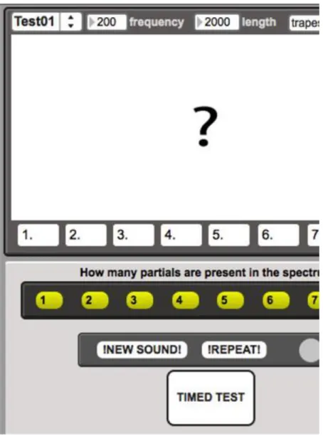
Figure 1.6. Test01

(14)

In Test01 you can test your skills gained in Excercise1 (Ex01). The interface is similar but the amplitudes of the partials are hidden. Press the button ’!NEW SOUND!’, and the patch will randomly play you one of the eight spectra. As an answer you have to select the corresponding yellow button. The correct answer is indicated by the green Led in the bottom right corner. If the answer is incorrect, it will be red and you can guess again. If you need to hear the sound again, press the ’!REPEAT!’ button.

Try this test with different fundamental frequencies, lengths and envelopes.

After you practiced, tested yourself and feel confident in indentifying the combinations of partials, you can move on to the timed test by clicking on the button.

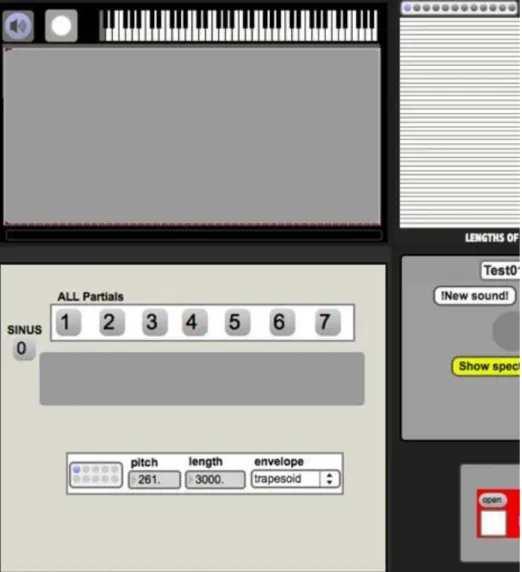
Excercise2 (Ex02)

Figure 1.7. Ex02

(15)

Excercise 2 (Ex02) offers seven different spectra. The partials are added to the fundamental from the top. By pressing the yellow button labelled "1+8" you will hear the fundamental and the 8th partial. Pressing button

"1+7-8" you will hear the fundamental with the 7th and 8th partials and so on . Pressing the button ’all’ you will hear the fundamental with all 7 overtones. This is like pressing button 8 in Ex01. Listen and try to memorize the eight spectra!

Excercise3 (Ex03)

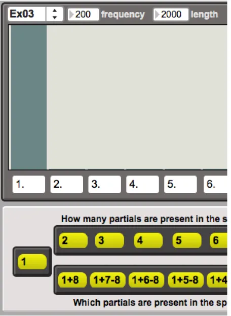
Figure 1.8. Ex03

(16)

Excercise3 (Ex03) combines Ex01 and 02. The circular setup of the buttons illustrates a continuous timbre scale.

Listen and try to memorize the 14 spectra!

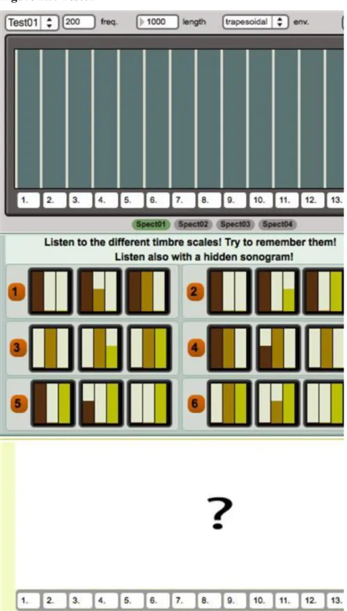
Test02

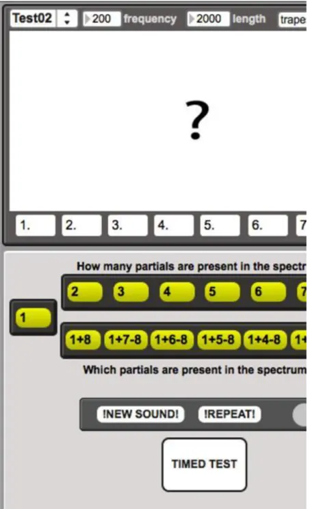
Figure 1.9. Test02

(17)

In this excercise you can test your skills gained in Excercises 2 and 3. The test functions as in Test01.

Excercise4 (Ex04)

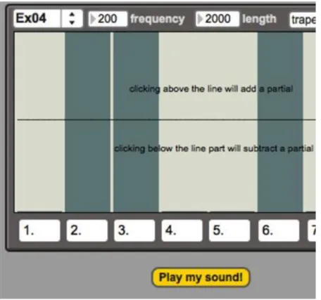
Figure 1.10. Ex04

(18)

In Excercise4 any combination of the eight partials is possible. Because the number of these combinations is huge, using yellow button for each possible combination would be unpractical. Therefore you need to click in the space directly above the number box to trigger the fundamental and its harmonics. Try to memorize the sounds resulting from different combinations of partials.

Test03

Figure 1.11. Test03

(19)

In Test03 you need to identify different combinations of the eight partials. Pressing the button ’!NEW SOUND!’

will play you a random set. On the screen with red columns you should select the partials you think are present in the perceived sound. You can check your result by clicking on the ’Play my sound!’ button. To compare your result with the test sound, you should click the ’!REPEAT!" button and again the ’Play my sound!’ button as many times as you need. To see, how close you are to the right answer, you should click on the ’Show Result!’

button, which will give you the result in the right lower corner as a percentage.

Pressing the button ’Show spectrogram!’ will show you the partials present in the test sound on the upper screen so that you can see any differences.

2.3. Listening strategies

We tend to hear harmonic timbre as a whole. The purpose of this lesson is to encourage you to develop more

(20)

Everybody hears the spectrum quite subjectively, so it is important to find personal strategies to identify the sonorities. To remember a sound it is important to name, identify and categorize it thru association and comparison (e.g. this sound reminds me of cicadas at the sea). This is a useful starting point, which needs to be refined with more analytical hearing. Here are three strategies to follow to increase your ability to understand what's happening in the sounds presented in this chapter:

1. Listen to the timbre as an overall sound. The fundamental sinewave (button 1) is easy to identify for its purity and emptiness. The sound becomes warmer thru adding the lower partials (2,3,4). When the higher partials are added (5 and above) depending on the fundamental frequency the sound becomes more nasal or harsher or more metallic.

2. Train your ear to hear the highest partial, because it will help you to recognise the full spectrum. Listen to the partials individually and try to remember their pitch compared to that of the fundamental. As we ascend, the pitches of the partials will follow the scale of the overtones (see fig. 1.2.).

3. Pay particular attention to the intervallic distance between the two top partials. The interval between each successive partial becomes smaller and therefore more dissonant. So partials 7 and 8, for example, will create a noticable dissonance or harshness in the sound.

It is important to remember that the frequency of the fundamental will greatly influence the perception of the resulting sound.

• at 120 Hz and below, the partials fall into separate critical bands so it is easier to hear them separately and the intervals can be heard more clearly.

• for higher sounds (150-500 Hz) where some of the partials fall within the same critical bands you should concentrate more on hearing any dissonance present in the sound, any roughness any nasal or metallic character.

To practice the fusion of 8 sinewaves, start with the trapesoidal envelope, a length of 2000 msec or more and a relatively low fundamental frequency (80 to 250 Hz). Higher, shorter and percussive sounds tend to fuse more completely, therefore it is harder to distinguish the partials within the sound.

(21)

Chapter 2. Superposition of sinewaves II. – Tri-stimulus

1. Theoretical background

The Tri-stimulus method is one of a number of representational approaches for understanding the perception of the harmonic spectrum of a sound. The theory was proposed by Pollard and Jansson¹ as an analogy of trichromatic color-vision/perception. (When light enters the eye, it falls on three different types of receptor cone cells that are tuned to the wavelengths or frequencies of red, green and blue light, the brain combines the information from each type of receptor to give rise to the perception of different wavelengths of light, or colours).

Similarly, the main properties of harmonic sound spectra can also be reduced to three parameters that correspond to specific spectral regions of the sound. Region 1 is the fundamental (1st partial). Region 2 contains the mid-range partials 2-3-4, and Region 3 contains the higher-range 5th partial and upwards. The ratio of the average loudness of each region can be represented within a triangular shaped coordinate system that is known as the tristimulus diagram (see Fig. 2.1.). If we add together the three regions, the result equals 1. The horizontal axis represents the mid range frequencies (m), the vertical axis, the higher range frequencies (h), the remaining part will equal the fundamental. So that, f + m + h = 1.

A pure sinewave with no harmonic partials is represented by a point at (0,0). Since the loudness value of the frequencies of middle and higher partials = 0, the loudness value of the fundamental =1. A sound where the timbre is balanced is represented by the black dot in the middle of the triangle, the value of the loudness of the mid and high partial groups is equal (m/3 + h/3 + f/3 = 1). The yellow and red dots represent the tristimulus positions of a violin and an oboe respectively. The more balanced timbre of the violin has slightly more higher partials than mid-range partials. The oboe has predominantly more mid-range partials in its spectrum. The curved green line indicates a sound where the ratio of the loudness of mid and high range partials changes over time.

Figure 2.1. tristimulus diagram

(22)

Superposition of sinewaves II. – Tri- stimulus

2. Practical Exercises

In this chapter we will use SLApp02.1 and SLApp02.2 to further explore harmonic spectra using the tristimulus method.

SLApp02 (containing SLApp02.1 and SLApp02.2) is downloadable for Windows and Mac OS X platforms using the following links: SLApp02 Windows, SLApp02 Mac OS X.

2.1. Using SLApp02-1

With SLApp02-1 (Fig. 2.2.) you can create and listen to different tristimulus variations of a source sound created from 16 sinewaves by changind the position of the grey dot in the triangle.

Figure 2.2. Layout of SLApp02-1

(23)

2.2. How SLApp02-2 works

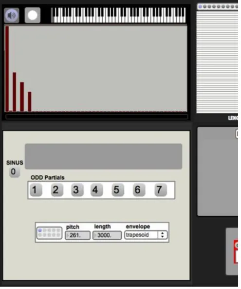
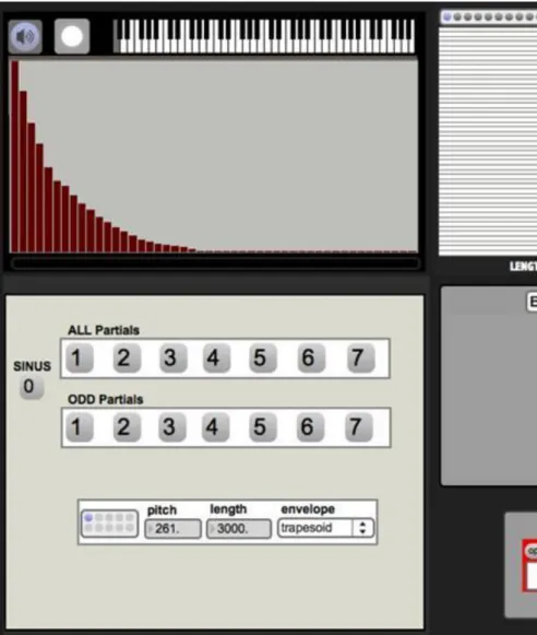
Figure 2.3. Layout of SLApp02-2

(24)

1. Selection of excercises - in the pop-down menu four excercises and three tests can be selected.

2. Frequency- here the fundamental frequency (first partial) is displayed. It can be changed by clicking and dragging or entering numbers.

4. Amplitude envelope - in the pop-down menu three types of amplitude envelopes can be selected: trapesoid, triangle, percussive.

5. Play the sound 6. Sound On-Off button.

(25)

7. Spectrum of the source sound

Sixteen green columns represent the amplitude of the partials. These can be changed by clicking and dragging. The number boxes below indicate the frequency ratio of the partials. they are fixed at the fundamental and the first 15 harmonics.

8. Source sound selector

Different spectra can be selected by clicking on the buttons:

Spect01 - all partiall with full amplitude Spect02 - odd partials with full amplitude

Spect03 - odd partials with decreasing amplitudes at higher harmonics Spect04 - random spectra

9. Preset buttons

By pressing the buttons you can select and hear a spectrum created using tristimulus combination. The coloured columns represent the relative amplitudes of fudamental, mid-range, and high-range partials.

10. Buttons to hide or show the spectrum of the transformed source sound (11) 11. Spectrum of source sound transformed by tristimulus presets (9)

2.3. Using SLApp02-2

These are series of exercises and tests, which will help you to become familiar with the harmonic spectrum represented by the three tristimulus regions.

In Excercise01 only two regions of partials are used. In Excercise02 all three regions are used which offer more cominations and complex sounds.

In all presets (9) the relative levels of the tristimulus regions are set at maximum, half or zero level. This limits the possible timbral combinations allowing you to concentrate on the basics.

The upper sonogram-like display represents the spectrum of the source sound, and the result of the tristimulus transformation can be seen on the lower display. Even more combinations can be created by changing the amplitude levels of the partials in the source spectrum.

Excercise1 (Ex01)

Figure 2.4. Ex01

(26)

In Ex01 by clicking on the numbers on the left side of the 3 part scales you will hear 3 sounds representing 3 combinations of regions in sequence. The spectrogram below changes to indicate which combination is playing, helping you to identify the sounds visually. Clicking on the ’Hide spectrogram!’ makes the exercise more difficult by removing it. Listen and try to memorize the different scales!

You can also click on the preset buttons to hear them individually. Listen and try to memorize the presets the different tristimulus combinations!

Test01

(27)

Figure 2.5. Test01

When you've spent some time listening to the scales in Ex01 you can test your listening skills here with Test01.

Press the button ’!New scale!’ the patch plays one of the six scales from Ex01. See if you can recognize them.

To answer click on the corresponding orange number button. The correct answer is indicated by the green Led in the bottom right corner. If the answer is incorrect, it will be red and you can guess again. If you need to hear the sound again, press the ’!REPEAT!’ button. To see the spectra of your answer press the ’Show spectrogram!’

(28)

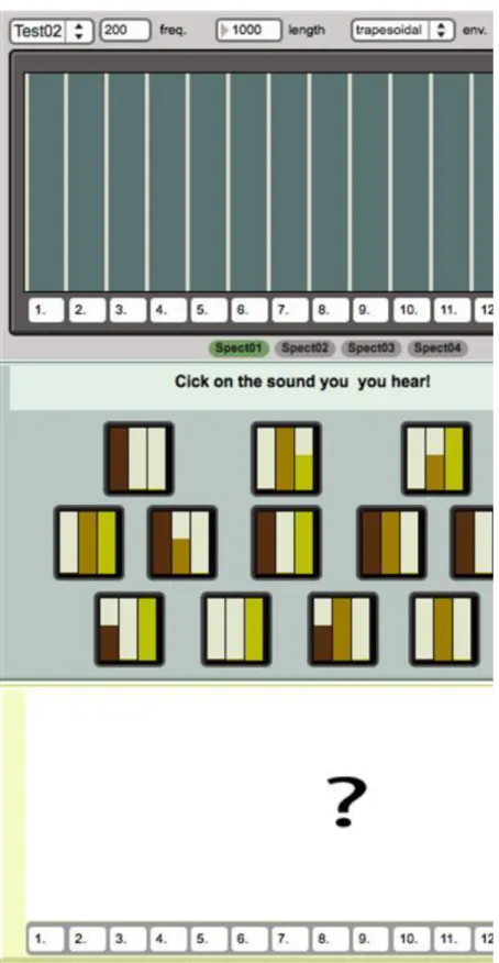
Test02

Figure 2.6. Test02

In Test02 the presets arre arranged randomly not in scaled as they were in Ex01 and Test01.

Press the button ’!New sound!’. To answer click on the corresponding preset button. The correct answer is indicated by the green Led to the right of the central panel. If the answer is incorrect, it will be red and you can

(29)

guess again. If you need to hear the sound again, press the ’!REPEAT!’ button. To see the spectra of your answer press the ’Show spectrogram!’ button.

Excercise2 (Ex02)

Figure 2.7. Ex02

(30)

Ex02 introduces the third region, so you can practise with a combination of all three. Sixteen different possible timbre combinations can be selected by clicking on the preset buttons. Listen and try to memorize the different combinations!

Test03

Figure 2.8. Test03

(31)

Test03 tests your ability to hear and differentiate between the combinations of three-partial regions explored in Ex02. The test interface functions exactly as in Test02.

2.4. Practicing strategies for tristimulus

The three regions of the tristimulus representation include three different types of sonority:

• f0, the fundamental sinewave has an empty, pure sound without any roughness or beating. Because of its low frequency, it will "darken" the timbre of a spectrum, it could be said to add power to the resulting timbre. Try listening to the difference of the spectrum with and wihtout the fundamental.

• the middle region – the 2nd, 3nd, 4th partials – creates resolved, pleasant intervals (octaves and fifth).

Compared with the simplicity of the fundamental sinewave this region according to Helmholtz is "rich and splendid but because of the absence of the higher partial is still soft and pleasant. Try listening to the difference of the spectrum with and wihtout the middle region.

• in the highest region the partials are much closer to each other creating smaller intervals. Above the 6th partial the intervals between the consecutive overtones are smaller than a major second and ascending higher they become more and more dissonant. In this region the tone becomes cutting, shrill, buzzing or rough depending on the frequency of the fundamental. Try listening to the difference of the spectrum with and wihtout the high region.

Listen to the individual spectral regions defined by the tristimulus representation, to learn to differentiate between the three kinds of percepts. After being able to identify each of them in different pitch regions, try their combinations.

(32)

Chapter 3. Superposition of

sinewaves III. – Transitions between waveforms

In this chapter we will explore the perceptual differences between spectra exhibited by some familiar waveforms: sine wave, triangle wave, square wave and sawtooth wave.

As in chapters 1 & 2, the spectra are created by adding sinewaves together (additive synthesis), but now we have many more partials. Spectra made up of 48 sinewaves are rich enough to test the differences between the above mentioned types of waveform.

1. Theoretical background

A sinewave is a smooth repetitive oscillation, which cannot be created by summing other types of waveforms. It is the simplest building block to describe and approximate any periodic waveform.

The shape of a sine wave can be described by its:

• frequency (f) that is the number of the repeating cycles in one second,

• amplitude (A) that is the peak deviation from the central middle level in each direction,

• phase (ph) that is the initial angle of a waveform at its origin.

Frequency and amplitude define the sound that we hear, phase has no affect on the auditive result. The pitch of a sine wave depends on the frequency, the loudness depends on the amplitude of the wave. (The greater the frequency, the higher the pitch; the bigger the amplitude, the louder the sound and vice versa.)

When adding together sine waves which are in harmonic relation to each other, more and more complex periodic waveforms will result (e.g. triangle or sawtooth) the spectra of which can be defined by simple rules.

The timbre of these waveforms are very characteristic, that's why they were chosen as the building blocks of many synthesizers.

Sawtooth wave is a complex, non-sinusoidal waveform that contains all the integer harmonics (f, 2f, 3f, 4f, etc.) with equal intensity. The sound is harsh and clear. The name of this wave was given after the shape of the sum of sine waves (see Fig. 3.1.).

Figure 3.1. sawtooth wave - http://en.wikipedia.org/wiki/File:Synthesis_sawtooth.gif

Triangle and square waves are complex waveforms in which the spectra contain only the odd numbered partials (f, 3f, 5f, 7f, etc.). Both waveforms are named after their shape. Square wave is similar to triangle wave since it also contains the odd numbered partials. The higher harmonics of a triangle wave roll off much faster than in a square wave (proportional to the inverse square of the harmonic number as opposed to just the inverse).

The shape of a triangle wave (and the square wave) can be seen in Fig. 3.2. and 3.3.

Figure 3.2. triangle wave

(33)

Superposition of sinewaves III. – Transitions between waveforms

Figure 3.3. square wave

To summarize:

• Sinewave: the simplest form which can not be subdivided any more

• Sawtooth wave: non-sinusoidal, contains all the partials: (f, 2, 3, 4, 5, 6 etc.)

• Triangle wave: contains only the odd numbered partials: (f, 3, 5, 7, 9 etc.)

• Squarewave: contains only the odd numbered partials: (f, 3, 5, 7,9 etc.) You can listen to the four basic soundtype here:

3.1 Sound - Sinewave 3.2 Sound - Sawtooth wave 3.3 Sound - Triangle wave 3.4 Sound - Squarewave

The aural difference between the spectra of the sine wave, the sawtooth wave and the triangle wave is quite obvious. It is clear that sine wave is a pure sound. The triangle wave with the odd numbered harmonics has a hollow, clarinet like sound. The sawtooth is the most complex sound being richer and nasal.

We can create interpolations between waveforms by changing the amplitudes of their partials. In this way a continuous timbre scale can be built up between the sine and the other waveforms (triangle, sawtooth, square).

2. Practical Exercises

2.1. How SLApp03 works

Figure 3.4. structure of the patch

(34)

1. Fundamental frequency – keyboard

The fundamental frequency of the spectra can be selected here pressing the keys of the keyboard. The spectrum will be specified by the multiplication of this frequency by integer numbers between 1-48.

2. Play the specified sound

Pressing the button the specified sound is played.

4. Spectrum of the sound

Fortyeight red columns represent the amplitude of the partials. These can be changed by clicking and dragging.

Amplitude envelope - in the pop-down menu three types of amplitude envelopes can be selected: trapesoid, triangle, percussive.

6. Preset buttons selecting different spectra (100 Hz)

Pressing the buttons you can play the sounds from sine-wave to total spectrum at 100 Hz fundamental frequency.

Pressing the buttons you can play the sounds from sine-wave to total spectrum at 200 Hz fundamental frequency.

(35)

Pressing the buttons you can play the sounds from sine-wave to total spectrum at 400 Hz fundamental frequency

9. Record the sound

Pressing the ”open” button, naming the file and clicking on the record button you can record the created sounds. Afterwards stop the recording by pressing the recording button again.

10. Selection of excercises - in the pop-down menu four excercises and four tests can be selected.

11. Length of the individual partials

The horizontal axis corresponds to the overall duration of the sound. The lines represent the individual partials with the fundamental at the bottom and the highest partial at the top.

Click on the preset buttons above for twelve combinations of the duration of each partial and you can click and drag in the panel to change the lengths of the partials.

We suggest you use this timbral dimension only after you have become familiar with the preceding exercises.

2.2. Using SLApp03

These are series of exercises and tests, which will help you to become familiar with the sound of the sinewave, the sawtooth and the triangle and the transisions between them.

In all examples the button marked 0 in the panel (at 8) triggers the fundamental sinewave. Buttons 1 thru 7 add more partials.

Ex01

Figure 3.5. Ex01

(36)

In Exercise1 (EX01) you can explore the transition between sinewave and sawtooth wave (all partials present).

The button marked 0 in the panel (at 8) triggers the fundamental sinewave. Buttons 1 thru 7 add more partials.

Listen and try to memorize the 8 spectra!

You may experiment with different fundamental frequencies, lengths and envelopes as well.

Test01

Figure 3.6. Test01 Test your ability to hear the transition between the sinewave and the

sawtooth wave introduced in Ex01.

(37)

Press the button ’!NEW SOUND!’ to hear one of the eight spectra. To answer click on one of the numbered buttons (0-7). The correct answer is indicated by the green Led in the bottom right corner. If the answer is incorrect, it will be red and you can guess again. If you need to hear the sound again, press the ’!REPEAT!’

button.

Pressing ’Show spectrogram!’ will display the partials and their relative amplitudes (as in EX01).

Ex02

Figure 3.7. Ex02

(38)

In Exercise2 (EX02) you can explore the transition between sinewave and triangle wave (odd partials present).

Again the button marked 0 in the panel (at 8) triggers the fundamental sinewave. Buttons 1 thru 7 add more partials. Listen and try to memorize the 8 spectra!

You may experiment with different fundamental frequencies, lengths and envelopes as well.

Test02

As Test01 just for the triangle wave.

Ex03

Figure 3.8. Ex03

(39)

Exercise03 combines the sawtooth and the triangle wave. Here you can compare the difference between the character of the sound of the three waveforms (sinewave, traingle, sawtooth). Notice that in all transitional steps (1-7) you can hear the characteristics of the sawtooth and the triangle emerging.

Practice both sawtooth and triangle wave as in Exercises01 and 02. This time pay particular attention to the difference you can hear between the waveform types.

Experiment with different fundamental frequencies, lengths and envelopes.

Test03

As Test01 just for the combination of sawtooth and triangle wave.

Ex04

Figure 3.9. Ex04

(40)

In Ex04 you have an interface combining the spectra seen in Ex03, this time with three different fundamental frequencies (100, 200, 400 Hz). The purpose of this interface is to allow you to develop the ability to hear the number and amplitude structure of the partials independent of the fundamental frequency. It is important to understand the influence of pitch register in contributing to the timbral characteristic of sounds, as it tends to mask the characteristics of the different waveforms and transitions between them.

First become familiar with the transformation from sinewave (0) to sawtooth and triangle (7) for each frequency.

After that try listening "vertically" alternating different frequencies.

Test04

Figure 3.10. Test04

(41)

Test your ability to hear the transition between the sinewave and the sawtooth and/or trangle wave in different pitch registers.

Pressing "New sound!" will select sounds from any of the given fundamental frequencies and number of partials both odd and all.

The test functions exactly as in Test01.

2.3. Practicing strategies for identifying different harmonic spectra (sinewave, traingle, sawtooth)

To identify different harmoinc spectra it is suggested you pay particular attention to:

• the different "qualities" of the timbre: learn to identify the hollow, clarinet-like quality of the triangle wave and distinguish it from the nasal oboe-like sound of sawtooth wave. The difference is a result of the absence or presence of the even numbered partials.

• the presence of higher partial will influence the brightness of the sound. Remember the higher the partials the closer to each other they are, the more dissonant they are, the harsher the resulting sound. It will result in both spectra-types (triangle and sawtooth) in a buzzing or serrated quality in the sound.

In addition to listening and exploring the qualities of sound transformed by the amplitude and presence of odd or all partials we can significantly change teh quality of the sound by changing the overall length, the amplitude anvelope and the duration of individual partials. The length of the partials can be changed by clicking on the

(42)

Chapter 4. Superposition of

sinewaves IV. – Inharmonic spectrum

In the following chapters you will learn about the timbre of inharmonic spectra created from different numbers of partials in different combinations.

1. Theoretical background

An inharmonic spectrum contains frequency components whose frequencies are not integer multiples of the fundamental.

The closeness of the partials, their frequency ratio, the length and the amplitude of the partials defines the fusion and the sense of the given spectra. The inharmonic spectrum could be described as the transition between harmonic sounds (see Chapters 1-3) and noise (see Chapter 7). Whilest it is obvious what pitch is heard when a harmonic sound is played, with inharmonic sounds it is not so clear.

The difference between harmonic and inharmonic sounds can be perceived as sensory dissonance. The level of inharmonicity is dependent upon the distance between the partials of a sectrum. There are different degrees of inharmonicity ranging from beating through roughness to distinguishable intervals.

The well-known phenomenon of beating occurs when two sinewaves have frequencies which are very close to each other. When the two frequencies are between 1 and a few Hertz apart, our ears hear only one frequency with a periodacally changing amplitude. The speed of the beating corresponds to the difference between the frequencies of the two sinewaves. (Listen to the beating produced by two sinewaves with that are 1, 2, 4 and 10 Hz apart – 4.01_Sound.)

If the sinewaves are further from each other (approx. 10 Hz or more), we can no longer perceive the beating as separate amplitude peaks, they occur so fast, we hear them as a ”roughness”.

When the difference between the frequencies of the sinewaves is larger than the so called critical band, they will be heard separately and a percept of an interval or fusio will occur.

4.1 Sound

According to Beauchamp¹ inharmonic sounds have three categories:

1. Sounds with nearly harmonic partials 2. Sounds with widely spaced (parse) partials 3. Sounds with closely spaced (dense) partials

1.1. Sounds with nearly harmonic partials

The partials of this spectrum diverge slightly, but increasingly, from the harmonic partials so the higher the partial, the greater the divergence. Beating or plucking a string will produce a spectrum divergent from a clear harmonic one. This phenomenon results in a clearer, colder, more tense and brighter sound.

Figure 4.1. spectrum of nearly harmonic partials

1Beauchamp, James W.: „Analysis and Synthesis of Musical Instrumental Sounds”. In: James W. Beauchamp (ed.): Analysis and Synthesis, and Perception of Musical Sounds, The Sound of Music. New York: Springer Science+Business Media, 2007. 1-89.

(43)

Superposition of sinewaves IV. – Inharmonic spectrum

1.2. Sounds with widely spaced (sparse) partials

Since the partials are dispersed and are separat from each other, there is no ”roughness” between them. At the same time some partials could be in harmonic relation so they fuse better than others. This is typical for certain acoustic instruments (e.g. percussion with wooden or metal plates).

Figure 4.2. spectrum of widely spaced (parse) partials

1.3. Sounds with closely spaced (dense) partials

Since the partials are very close to each other, the roughness of the spectrum is very evident. Therefore no pitch content can be heard. Most metal plate or stretched membrane instruments sound this way. Their spectra might sometimes resemble that of white-noise (see Chapter 7). The sound of a suspended cymbal is a good example of

(44)

Figure 4.3. spectrum of closely spaced (dense) partials

2. Practical Exercises

2.1. How SLApp04 works

Figure 4.4. Layout of SLApp04

(45)

1. Fundamental frequency – keyboard and number box

The fundamental frequency of the spectra can be selected here pressing the keys of the keyboard and clicking and dragging the number box marked pitch. The spectrum will be specified by the multiplication of this frequency by teh numbers given at Partials.

2. Play the specified sound

Pressing the button the specified sound is played.

Amplitude envelope - in the pop-down menu three types of amplitude envelopes can be selected: trapesoid, triangle, percussive.

5. Spectrum of the sound

Fortyeight red columns represent the amplitude of the partials. These can be changed by clicking and dragging.

6. Frequency ratio of the 48 partials

The frequency ratio of each partial can be specified in the 48 number boxes. The buttons to the right will load presets of different partial ratios.

(Button1 – harmonic partials used for the beating. Buttons 2-5 – different inharmonic ratios with different

(46)

7. Preset buttons selecting different spectra with different spectral densities (By spectral density we mean the number of partials present in the spectrum).

8. Preset buttons selecting different spectra with different beating frequencies

9. Record the sound

10. Selection of excercises - in the pop-down menu three excercises and two tests can be selected.

11. Length of the individual partials

The horizontal axis corresponds to the overall duration of the sound. The lines represent the individual partials with the fundamental at the bottom and the highest partial at the top.

Click on the preset buttons above for twelve combinations of the duration of each partial and you can click and drag in the panel to change the lengths of the partials.

We suggest you use this timbral dimension only after you have become familiar with the preceding exercises.

2.2. Using SLApp04

Here we explore the phenomena of beating and different types of inharmonic spectra. The sounds that can be produced by inharmonic spectra are far more complex than those produced by purely harmonic ratios between the fundamental and its partials.

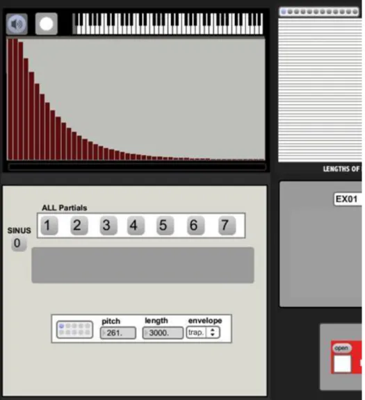
Ex01

Figure 4.5. Ex01

(47)

In this exercise you will explore a continuum from a pure harmonic spectrum (0) thru beating to roughness (7) as discussed earlier. The source spectrum is built from 48 partials with integer ratios. When transforming the source spectrum there are 2 sinewaves added above and below each partial. The difference between the frequency and amplitude of the partials and those of the added sinusoids will determine if we hear beating or roughness.

In the panel marked "Beating" there are two rows of buttons 1-7. In the top row the amplitude of teh added sinewaves is equal to the amplitude of the source partials. In the lower row the sinewaves are 0.3 of the amplitude of the source partials. The preset buttons 1-7 determine the frequency of the beating. In button 1 you can hear recognizable slow beating, in button 7 the beating is so fast that you hear it as beating. It is important to note that the values of the frequencies of the added sinewaves will vary randomly at each partial. The preset numbers will define the range of the randomness of the beating frequency in Hertz indicated in the panel below.

Button 1 adds beating with a frequency from 1 to 6 Hz, button 2 with 5 to 10 Hz, button 3 with 8 to 14 Hz, button 4 with 13 to 18 Hz, button 5 with 17 to 24 Hz, button 6 with 23 to 33 Hz and button 7 with 32 to 51 Hz.

These added sinewaves create a scale from soft beats to roughness.

You may change the fundamental frequency, the length and the envelope as well.

Test 01

(48)

Test your ability to hear and recognize the speed and amplitude of beating (roughness) introduced in Ex01.

Press the button ’!NEW SOUND!’to hear one of the fifteen possibilities. To answer click on one of the numbered buttons (0-7) in the two rows. The correct answer is indicated by the green Led in the bottom right corner. If the answer is incorrect, it will be red and you can guess again.

If you need to hear the sound again, press the ’!REPEAT!’ button. If you need to see the beating ranges, click on

"Show visuals!"

Ex02

Figure 4.7. Ex02

(49)

In this exercise now we explore inharmonic spectra with different spectral densities (ie. different number of partials of differing amplitudes present in the spectrum). The ratios of the partials to the fundamental can be seen in the central panel ranging from 1-10.72. Note that they are not integers and therefore the spectrum will be inharmonic.

There are two rows of 6 buttons. The top will trigger a fundamental frequency value of 200 Hz, the lower 100 Hz. By clicking on the buttons 1-6 you will see that each button triggers different combinations of partials of increasing density where 1 is the least dense and 6 is the most illustrating the difference betwwen sparse and dense spectra as discussed at the beginning of the chapter (Fig. 4.2. and 4.3.)

You can also practice with different spectra by selecting from the presets on the right side of the center Partial panel. You could set your own numbers by clicking and dragging the values.

Of yourse as always you can change the length of the sound, its amplitude envelope and the length of its partials.

Test02

The test works the same as in Test01.

Ex03

(50)

This exercise combines the possibilities of exploring beating and spectral density together. Play with it freely, create and record your own sounds. When you feel you found an exciting sound make sure you record the settings that have produced the sound. You could do this by using a screen grab.

(51)

Chapter 5. Modelling musical examples – bell-like sounds

In this chapter we will look at an analysis and a synthesis of a real world sound, that of a bell. It is a practical exercises, where you can explore how to model a bell like sound by adding inharmonic sinewaves together. You can also learn how to transform the sound radically by changing the amplitude envelopes of the individual partials.

1. Theoretical background

A well-known example of the fusion of inharmonic sounds is Jean-Claude Risset’s synthesized bell. Basically, the amplitude envelope of the spectrum of a bell has two phases; the initial attack phase is short, the release phase is much longer. The change in both of the phases is exponential. The difference between the two phases is that in the attack the partial envelopes are synchronised, while the partials release or fade at different rates. This behaviour was imitated by Risset creating independent sinewaves of different frequency, amplitude and length.

Table 5.1. frequency, amplitude and length ratios of Risset’s bell

Partial Frequency ratios Amplitude ratios Length ratios

11 7.2678 1.3429 0.0762

10 6.7142 0.9714 0.1048

9 5.3571 1.3429 0.1524

8 4.8928 1.3429 0.2

7 3.5714 1.4571 0.2476

6 3.1357 1.6571 0.1048

5 2.125 2.6857 0.3238

4 1.65 1.8 0.5524

3 1.6428 1 0.8762

2 1.0053 0.6857 0.9048

1 (fundamental) 1 1 1

The length or duration of the partials of a bell are different; generally, the lower ones are longer and this accounts for the sensation of a descending pitch when we listen to a bell. The amplitude envelopes are identical, but the amplitude ratios are different. The identical amplitude envelopes help the partials to fuse into one sound percept. Normally inharmonic spectra tend not to fuse as completely as harmonic spectra, but in this case because of the synchronized fast percussive attack the partials of the inharmonic spectrum of the bell sound like arriving from the same source.

You can see the basic parameters, frequency amplitude and length ratios, in the Table 5.1.

Risset not only created a synthesized imitation of a bell but he also exploited the independency of the partials to modify the sound. If the shape of the envelope is changed so that each partial has its dynamic climax point midway through its own duration, (5.2,c) the pitch of the actual partials will be heard at that point, creating an inharmonic falling melody. This also helps the listener to identify the individual partials that make up the sound of the bell. You can Risset's initial bell synthesis (both percussive and the transformation of the partial envelopes) at Sound_5.01.

Figure 5.1. a, b, c: partials and summing of bell-like sound with different envelopes

(52)

Modelling musical examples – bell- like sounds

(53)

5.1 Sound

Listening to the sound examples (5.02, 5.03,5.04) you can hear that the transformation caused by the change of form of the amplitude envelope creats similar effects in both harmonic and inharmonic spectra.

5.2 Sound - harmonic spectra

5.3 Sound - inharmonic spectra

5.4 Sound - inharmonic spectra

2. Practical Exercises

2.1. How SLApp05 works

You will notice the numbering system has changed a little because SLApp05 is more complex having more control parameters.

Figure 5.2. structure of the patch

(54)

2. Play sound button.

3. Selection of the excercises – in the pop-down menu two excercises can be selected.

4. Length – displays the duration of the sound. By clicking and dragging or entering numbers the value can be changed.

5. Frequency – the fundamental frequency can be changed here.

6. Amplitude envelope

In SLApp05 for the first time one can manipulate the amplitude envelope. When you open the SLApp by clicking on the preset buttons above you can move the peak form the beginning to the end. This envelope is applied to each partial over its duration.You can click and drag on the points on the envelope curve to create your own amplitude envelopes.

7. 7, 8, 9 – the length, amplitude and frequency ratios are displayed here and can be changed by clicking and dragging.

8. 10 – a 7x7 matrix of presets

The 49 buttons trigger different envelope and length values. The amplitude envelope can be changed by pressing the buttons on the horizontal axis as represented along the bottom in the form percentage of time.

The individual length of the partials can be changed by pressing the buttons on the vertical axis. On the right side of the matrix is a graphical representation of teh length ratios of the partials for each row.

9. 11 – Record the sound

(55)

2.2. Using SLApp05

Practice the fusion of inharmonic spectra by changing the length and amplitude of partials (based on Risset’s bell). The examples offer two different ways of practising based on different amplitude envelopes.

Ex01

Figure 5.3. Ex01

This excercise has envelopes with 7 different peak positions (0.1%, 2%, 5%, 8%, 11%, 14%, 20%). The peaks

(56)

Ex02

Figure 5.4. Interface of exercise2

This excercise has also 7 envelopes with different peak positions (0.1%, 10%, 30%, 50%, 65%, 80%, 99%). the peaks shift from the beginning (0.1%) to the end (99%) which determines wheather we hear a fused bell-like sound or a melody of the partials.

2.3. Practising strategies for hearing the fusion of partials of Risset’s bell

There are no tests in this chapter. We encourage you to play experiment and explore.

(57)

Since there are only two timbral dimensions changing in this patch it is worth concentrating on them one by one.

Learn the attack peaks and listen carefully to the softening of attack in Excercise1 and the emerging ”melodic”

phenomenon in Excercise 2 as the attack time becomes longer.

The phenomenon of fusion is more obvious with short and hard attacks. Partials are heard separately when their attack phases are longer. Where the length of the individual partials differ from the others each partial is heard separately.

(58)

Chapter 6. Modelling musical examples – endless scale and glissando

In the previous chapters the phenomenon of fusion has been central to our understanding of harmonic and in harmonic spectra. Here we will explore an interesting property which can be used to fool the ear completely.

In this chapter we will introduce the auditory illusion of the Shepard tone and the Shepard-Risset glissando. We think we hear endlessly rising or falling scales. It is fusion that is responsible for this illusion.

1. Theoretical background

The basis of this illusory phenomenon was invented in 1964 by Roger Shepard hence it is known as the Shepard tone. What we hear is a repeated set of tones organized in an ascending or descending scale. Once the ascent or descent is completed the sequence begins again. These tones are harmonic sounds made up of several partials.

As they step up or down the scale Shepard changed the amplitude of the individual partials of each tone. Each partial follows an amplitude curve so that it is its loudest at the midpoint of the pitch ascent/descent, and at is inaudible at the beginning and end of the ascent/descent (see Fig. 6. 1.). Because the partials are harmonically related they fuse into a single timbre. And because each partial is louder at its midpoint, it continously draws out attention to the middle register. By really concentrating and pulling your away from this loudest midpoint you can hear the beginning and end of the scale as it fades in and out.

Figure 6.1. visualisation of endless scale (also called Shepard’s scale)

(59)

Modelling musical examples – endless scale and glissando

Similarly our visual perception can be tricked by the Penrose staircase (see Figure 6.2.) which appears to fold back upon itself in space. This was the inspirational source for the familiar litograph by M. C. Escher’s Ascending and descending (http://en.wikipedia.org/wiki/Ascending_and_Descending).

Figure 6.2. Penrose staircase

(60)

While Shepard’s musical example is based on the discrete steps of a scale, Risset created a continuously sliding glissando, often called as Shepard-Risset glissando. The partials fuse in exactly the same way creating the illusion of an endless glissando (see Fig. 6.3.).

Figure 6.3. sonogram of endless glissando (also called Risset’s endless glissando)

2. Practical Exercises

(61)

2.1. How SLApp06 works

Figure 6.4. layout of SLApp06

1. Direction of scale/glissando

Select ascending or descending scale/glissando.

2. Length of period

The period is the duration of one cycle of ascent/descent

3. Lowest frequency of the spectrum – can be set between 20 and 200 Hz.

4. Interval between partials

The interval between the frequencies of partials in semitones from 1 to 15.29 5. Number of partials

Number of partials present (1 to 10).

6. Volume

8. Spectrogram/Sonogram – toggle between spectrogram and sonogram display

(62)

10. Partial amplitude envelope presets and display

Five amplitude envelope presets can be selected for the partials.

11. Amplitude envelope of fused sound (only for Shepard scale and not the glissando).

Percussive, end-peak and trapesoid envelopes can be selected.

12. Time interval

Interval between tones in Shepard scale (only works in periodoc mode). It can be set between 100 and 1000 msec.

13. Periodic/Continuous toggle

You can select between continuous (Risset’s endless glissando) and periodic (Shepard’s scale) sound.

14. Preset button triggering different parameter combinations influencing Shepard scale and Risset glissando

2.2. Practicing strategies

There are no special exercises or tests in this SLApp. When you first launch it, you will hear an ascending Shepard scale. Notice that there are eight partials each an octave (12 semitones) apart. Try changing the different parameters to see how they affect the illusion of endless ascent. Change to preset 2 (at 14) to hear what happens if we have only 2 partials present and the lowest frequency of the spectrum is 200 Hz. Listen to the beginning and the end of the sequence. Notice that the fusion and so the illusion is lost.

To hear the same effect with Risset glissando press prests 3 then 4.

Experiment and try altering different parameters of the SLApp. Pay particular attention to the partial amplitude envelope settings and how these are crucial in influencing the fusion. Also the harmonic reltionship of the partials will greatly influence whether or not we hear the partials fused in the glissando sequence. Find out the least number of partials necessary for the illusion.

(63)

Chapter 7. Filtering white noise with low-pass and high-pass filters

In the following chapters you will learn about synthesis based on filtering, known as subtractive synthesis.

This type of synthesis is the opposite of additive synthesis used in the first chapters. In additive synthesis, complex sound is created by adding simple waveforms together. Conversely, in subtractive synthesis, the starting point is a relatively complex waveform from which parts of the sound are removed by a process known as filtering. White noise (Fig.7.1, Sound7.1) is a useful starting point because it contains all frequencies, which we are going to filter in the following three SLApps.

Figure 7.1. sonogram of white noise

7.1 Sound

1. Theoretical background

1.1. Subtractive synthesis

A synthesis technique in which parts of the spectrum are subtracted by filtering. A filter is a device that performs some sort of transformation on the spectrum of a signal.

The most common types of filters are:

(64)

Filtering white noise with low-pass and high-pass filters

Figure 7.2. sonogram of low-pass filtered white noise

2) High-pass filter (Fig. 7.3.): passes the partials above a given cutoff frequency (or cuts the partials below it).

Figure 7.3. sonogram of high-pass filtered white noise

(65)

Filtering white noise with low-pass and high-pass filters

3) Band-pass filter (7.4.): passes the partials around the given centre frequency in the range of a given bandwidth.

Timbre Solfege

Timbre Solfege

Balázs Horváth

Andrea Szigetvári

Timbre Solfege

Table of Contents

List of Figures

List of Tables

Chapter 1. Superposition of sinewaves I.

1. Theoretical background

1.1. Harmonic spectrum

Figure 1.1. overtone system (the frequency values are rounded to integer numbers)

Figure 1.2. first eight partials of a harmonic sound

1.2. Fusion

2. Practical Exercises

2.1. How SLApp01 works

Figure 1.3. layout of SLApp01

Figure 1.4. layout of Timed Test

2.2. Using SLApp01

Figure 1.5. Ex01

Figure 1.6. Test01

Figure 1.7. Ex02

Figure 1.8. Ex03

Figure 1.9. Test02

Figure 1.10. Ex04

Figure 1.11. Test03

2.3. Listening strategies

Chapter 2. Superposition of sinewaves II. – Tri-stimulus

1. Theoretical background

Figure 2.1. tristimulus diagram

2. Practical Exercises

2.1. Using SLApp02-1

Figure 2.2. Layout of SLApp02-1

2.2. How SLApp02-2 works

Figure 2.3. Layout of SLApp02-2

2.3. Using SLApp02-2

Figure 2.4. Ex01

Figure 2.5. Test01

Figure 2.6. Test02

Figure 2.7. Ex02

Figure 2.8. Test03

2.4. Practicing strategies for tristimulus

Chapter 3. Superposition of

sinewaves III. – Transitions between waveforms

1. Theoretical background

Figure 3.1. sawtooth wave - http://en.wikipedia.org/wiki/File:Synthesis_sawtooth.gif

Figure 3.2. triangle wave

Figure 3.3. square wave

2. Practical Exercises

2.1. How SLApp03 works

Figure 3.4. structure of the patch

2.2. Using SLApp03

Figure 3.5. Ex01

Figure 3.6. Test01 Test your ability to hear the transition between the sinewave and the

sawtooth wave introduced in Ex01.

Figure 3.7. Ex02

Figure 3.8. Ex03

Figure 3.9. Ex04

Figure 3.10. Test04

2.3. Practicing strategies for identifying different harmonic spectra (sinewave, traingle, sawtooth)

Chapter 4. Superposition of

sinewaves IV. – Inharmonic spectrum

1. Theoretical background

1.1. Sounds with nearly harmonic partials

Figure 4.1. spectrum of nearly harmonic partials

1.2. Sounds with widely spaced (sparse) partials

Figure 4.2. spectrum of widely spaced (parse) partials

1.3. Sounds with closely spaced (dense) partials

Figure 4.3. spectrum of closely spaced (dense) partials

2. Practical Exercises

2.1. How SLApp04 works

Figure 4.4. Layout of SLApp04

2.2. Using SLApp04

Figure 4.5. Ex01

Figure 4.7. Ex02

Chapter 5. Modelling musical examples – bell-like sounds

1. Theoretical background

Table 5.1. frequency, amplitude and length ratios of Risset’s bell

Figure 5.1. a, b, c: partials and summing of bell-like sound with different envelopes

2. Practical Exercises