Thermoelastic analysis of layered disks

THERMOELASTIC ANALYZIS OF LAYERED DISKS

PhD student

Institute of Applied Mechanics, University of Miskolc, Miskolc, Hungary

Abstract: The main objective of this paper is the evaluation of the normal stresses and displacements in layered disks, which are caused by thermal and mechanical loadings. The analytical solutions for the temperature field and the corresponding thermal stresses are determined by utilizing the equations of the steady-state heat conduction and field equations of thermo-elasticity when the temperature and the displacement field depend only on the radial coordinate.

1. INTRODUCTION

This paper investigates a thermoelastic problem of a layered disk which has the inner radius of R₁, the outer radius is R_n+1, the thickness is denoted by 2m and n is the number of layers as Fig. 1 indicates. The layers of the thin structural component are perfectly coupled. In order to solve this problem a cylindrical coordinate system (rφz) is used. The radial stresses, the heatflow and the temperature are all continuous functions of the radial coordinate r.

The temperatures of the cylindrical boundary surfaces are given, they are constant, non time dependent and denoted by t_in and t_ou and there is convective heat exchange on the lower and upper plane boundary surfaces. It follows that the temperature field T(r) is the function of the radial coordinate. The uniformly distributed mechanical loading exerted on the inner boundary surface is denoted by -f₁=p_in, while -f_n+1=p_ou is the pressure which acts on the outer cylindrical boundary surface.

Figure 1. The sketch of the layered disk

Both the boundary conditions and the field equations [1,2] are linear, therefore the superposition principle can be used. This means that we can add the stresses and displacements caused by mechanical loads to the thermal stresses and displacements in order to solve the coupled problem of mechanical and thermoelasticity.

2. FORMULATION OF THE THERMOELASTIC PROBLEM

At first we consider the case when the i-th layer is under thermal loading and has a steady-state temperature field. The stresses on the curved boundary surfaces of the layers have zero values.

Figure 2. The cross section of a quarter of the i-th layer The u_i^T(r) thermal radial displacement and the σirT

(r), σiφT

(r), σiϑT

(r) thermal stresses can be formulated as [2]:

2 2 1

2 2

1

1 (1 ) (1 )

( ) ( ) ( ) ,

( )

i

i i

r R

T i i i i

i i i i i

i i

R R

R r

u r r r dr r r dr

r r R R

      ^ 



   

 





2 1

2 2 2 2

1

( ) ( ) 1 ( )

i

i i

r R

T i i i i i

ir i i

i i

R R

E E R

r r r dr r r dr

r R R r

 

  ^ 



 

 





2 1

2 2 2 2

1

( ) ( ) ( ) 1 ( )

i

i i

r R

T i i i i i

i i i i i i

i i

R R

E E R

r r r dr E r r r dr

r R R r



 

    ^ 



 







In the previous expressions E is the Young modulus,  is the Poisson ratio, α is the coefficient of linear thermal expansion and τi(r) is the function of temperature difference compared to a t_ref reference temperature of the i-th layer.

In the next step it is assumed that the inner and outer cylindrical boundary surfaces of the i-th layer are under constant mechanical loading f_i _ir^M( )R_i and

1 ^M( 1)

i ir i

f_  R_ . The differential equation of the radial displacement field, derived from the equilibrium equation:

2 2

2

( ) ( )

( ) 0

M M

i i M

i

d u r du r

r r u r

dr  dr   . (4)

The displacement field and the normal stresses have the following forms:

M( ) i

i i

u r A r B

  r , (5)

2

( ) 1

1 1

M i i i i

ir

i i

E A E B

r r

 ^  ^  , (6)

2

( ) ( ) 1

1 1

M M i i i i

i i

i i

E A E B

r r

  r

 

 

  

  , i1...n. (7) Using the equations for the boundary conditions, the unknown parameters A_i and B_i and the normal stresses can be determined:

2 2

1 1

2 2

1

(1 ) ( )

( )

i i i i i

i

i i i

R R f f

A E R R

 _{ }



 

  , (8)

2

1 1

2 2

1

( ) (1 )

i i i i

i i

i i i

R f f

B f

R R E

  



   

    , (9)

2 2 2

1 1 1 1

2 2 2 2 2

1 1

(1 ) ( ) 1 ( ) 1

( ) (1 )( ) 1

M i i i i i i i i i

ir i

i i i i i i

R R f f R f f

r f

R R R R r

 

  ^ _ ^  ^ _^

 

   

         , (10)

2 2 2

1 1 1 1

2 2 2 2 2

1 1

(1 ) ( ) 1 ( ) 1

( ) ( )

(1 )( ) 1

M M i i i i i i i i i

i i i

i i i i i i

R R f f R f f

r r f

R R R R r

 

 

 

 ^ _ ^  ^ _^

 

   

          ,i1,...,n.

(11)

3. SUPERPOSITION OF THE THERMAL AND MECHANICAL LOADS Considering the i-th layer for the computation of the radial displacement and radial stresses the following equations are used ():

( ) ^T( ) ^M( ),

i i i

u r u r u r (12)

( ) ^T( ) ^M( ),

ir r ir r ir r

   (13)

( ) ^T( ) ^M( ),

i_ r i_ r i_ r

   i1,..., .n (14)

The unknown f_i parameters in the equations of u_i^M(r), σirM

(r), σiφM

(r) can be calculated using equations

1 1 1

( ) ( ),

i i i i

u R_ u_ R_ i1,...,n1, (15) which ensures the continuity of the radial displacement field, furthermore f₁ and f_n+1 are given:

_1r(R₁) f₁ p_in, _nr(R_n1) f_n1 p_ou. (16)

The system of equations (16) can be expressed as

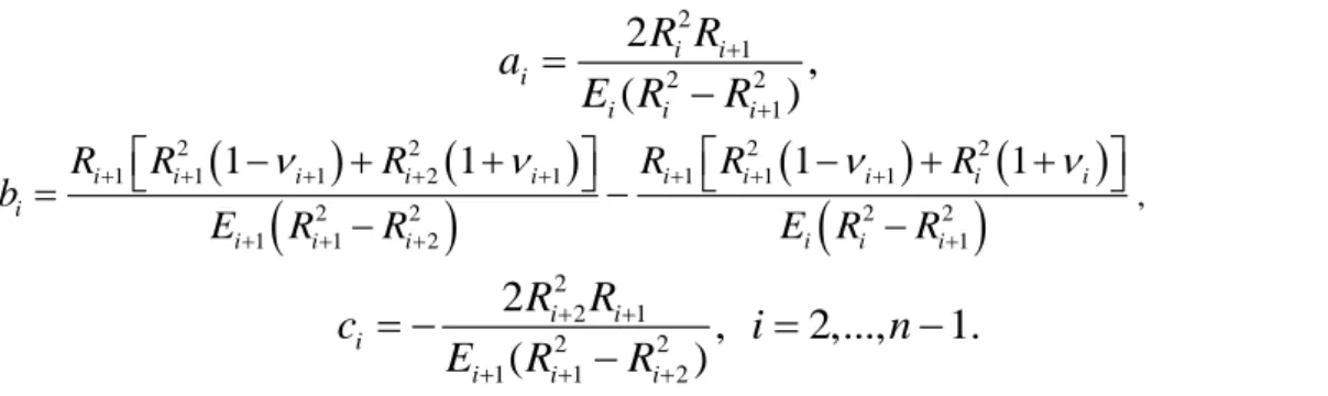
a f_{i i} b f_{i i1}c f_{i i2} u_i^T_1(R_i1)u_i^T(R_i1), i2...n1,(17) where the constants a_i, b_i and c_i have the following forms:

2 1

2 2

1

2 ,

( )

i i

i

i i i

a R R

E R R





  (18)

   

  ^  ^  ^{ }

2 2 2 2

1 1 1 2 1 1 1 1

2 2 2 2

1 1 2 1

1 1 1 1

i i i i i i i i i i

i

i i i i i i

R R R R R R

b E R R E R R

   

       

   

         

   

 

  ^, (19)

2

2 1

2 2

1 1 2

2 ,

( )

i i

i

i i i

c R R

E R R

 

  

   i2,...,n1. (20)

Using the previously determined f_i parameters and the equations (10-14) the radial displacement and the stresses of the layered spherical body can be evaluated.

4. DETERMINATION OF THE TEMPERATURE FIELD

The last step is the determination of the temperature field T=T(r). Figure 3 shows the sketch of the heat conduction problem. We assume that the temperature field is a continuous function of the radial coordinate and the enviromental temperature t_envi has zero value. By the previously mentioned thermal boundary conditions the differential equation of the heat conduction has the following form:

 

dr r dr

 q      , (21)

where

p h

m

 . (22)

Figure 3. The heat conduction problem

After solving Eq. (21), we get the temperature field of the i-th layer with the unknown integration constants:

T r_i( )C I_{i 0}(p r_i )D K p r_{i 0}( _i ), i1,...,n. (23) Using the boundary conditions C_i and D_i can be evaluated:

0 1 1 0

0

0 1 0 0 0 1

0 1 1 0

0

0 1 0 0 0 1

( ) ( )

( ) ( )

( ) ( ) ( ) ( )

( ) ( )

( ),

( ) ( ) ( ) ( )

i i i i i i

i i

i i i i i i i i

i i i i i i

i

i i i i i i i i

t K p R t K p R

T r I p r

K p R I p R K p R I p R t I p R t I p R

K p r K p R I p R K p R I p R

 

 

 

 

  



 

 

(24)

where I₀(x) and K₀(x) are the Bessel functions of the first and second kind and of order zero [3]. We consider the case when the radial heatflow is constant, the temperatures of the inner and outer boundary surfaces are given. The surface temperatures of the osculant layers are equal therefore we get the following equations:

1 ( 1) 1( 1)

i i i i i

t_ T R_ T_ R_ , q R_i( _i1)q_i1(R_i1), i1...n1, (25)

0 1 1 0

1

0 1 0 0 0 1

0 1 1 0

1

0 1 0 0 0 1

( ) ( )

( ) ( )

( ) ( ) ( ) ( )

( ) ( )

( )

( ) ( ) ( ) ( )

i i i i i i

i i i i

i i i i i i i i

i i i i i i

i i i

i i i i i i i i

t K p R t K p R

q r p I p r

K p R I p R K p R I p R t I p R t I p R

p K p r

K p R I p R K p R I p R





 

 

 

 

   



 

 

, i1,...,n, (26)

where λ_i is the thermal conductivity of the i-th layer. The unknown temperature values of the osculant boundary surfaces can be calculated using the system of equations (25-26).

5. NUMERICAL EXAMPLES

We consider a four-layered structural component. The layers of the disk are made of four different materials which are the different composition of the same two materials (steel-ceramic). For the numerical computation the following data are used:

1 2 3 4 4

1 2 3 2

6

1 2 3 4 1

6 6 6

2 3 4

0.05m, 0.055m, 0.06 m, 0.065m, 0.07m, 0.5mm,

223.7GPa, 249.5GPa, 275.8GPa, 302.4GPa,

0.297, 0.331, 0,366, 0.401, 1.27 10 1 ,

K

1 1 1

1.42 10 , 1.57 10 , 1.72 10 ,

K K K

R R R R R m

E E E E

h

    

  



  

     

   

     

      ₂

1 2 3 4

70 W , m K

W W W W

61.49 , 68.59 , 75.81 , 83.14 ,

mK mK mK mK

   



   

1 _in 20MPa. 5 _ou 0MPa, 1 273K, 5 473K, _ref 273K.

f  p   f  p  t  t  t 

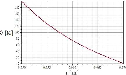
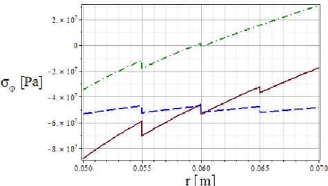
Figures 4-7 indicate the results of this problem, solved with Maple 15, in three cases. In Figs. 5-7 the green dashdot lines show the functions of the displacement field and normal stresses when there is only thermal loading (p_in=0MPa), the blue dash curves are the results of the mechanical load (ϑ(r)=0K) and the solid red lines illustrate the results for the original problem (thermal and mechanical loads).

Figures 4. The temperature difference function

Figure 5. The displacement fields

Figure 6. The radial normal stresses of the different cases

Figure 7. The tangential normal stresses 6. CONCLUSIONS

The main objective of this paper was to present an analytical solution for the displacement field and the associated stresses in thin layered disk subjected to mechanical and thermal loads. To solve this problem the Fourier’s law of heat conduction and the equations of thermal stresses with steady temperature field were used. The developed solution can be utilized as Benchmark solutions for numerical methods to verify the accuracy of the numerical methods. If we increase the number of the layers and discretize the function of the material properties for the different layers, the displacement field and the normal stresses of functionally graded disks can be calculated with this method.

Acknowledgements: This research was supported by the European Union and the State of Hungary, co-financed by the European Social Fund in the framework of TÁMOP-4.2.4.A/ 2-11/1-2012-0001 ‘National Excellence Program’.

REFERENCES

[1] Boley, B. A., Weiner, J. H.: Theory of Thermal Stresses, John Wiley & Sons Inc., New York, 1960.

[2] Nowinski, I. L.: Theory of Thermoelasticity with Applications. Sythoff and Noordhoff, Alpen aan den Rijn, 1978.

[3] Carslaw, H. S., Jaeger, I. C.:Conduction of Heat in solids, Clarendon Press, Oxford, 1959.