The determination of displacement field and normal stresses in multilayered spherical bodies

THE DETERMINATION OF DISPLACEMENT FIELD AND NORMAL STRESSES IN MULTILAYERED SPHERICAL BODIES

Gönczi Dávid PhD student

Institute of Applied Mechanics,University of Miskolc, Miskolc, Hungary Abstract: The main objective of this paper is the calculation of the thermomechanical stresses and displacements in layered spherical bodies subjected to thermal and mechanical loadings. It is assumed that the temperature field and the displacement field depend only on the radial coordinate. The exact solution of one layer is used to get the analytical solution for the whole layered body by fitting the displacement and stress values on the boundary surfaces.

1. INTRODUCTION

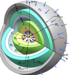
This paper investigates a thermoelastic problem of a hollow layered spherical body. The geometry of the investigated body can be seen in Fig. 1, where the inner radius of the sphere is R₁, the outer radius is R_n+1 and n is the number of layers. The layers of the spherical structural component are assumed to be perfectly coupled and made of homogeneous, isotropic materials, furthermore a spherical coordinate system (rφϑ) is used.

Figure 1. The three-dimensional sketch of the hollow layered sphere

First kind thermal boundary conditions are prescribed on the inner and outer spherical surfaces. These temperature values are given, they are assumed to be constant, non-time- dependent and denoted by t₁ and t_n+1. It follows that the temperature field T(r) is the function of the radial coordinate. The uniformly distributed mechanical loading exerted on the inner boundary surface is denoted by

f₁=p_i, while -f_n+1=p_o is the pressure which acts on the outer curved boundary surface.

It is assumed that the radial stresses, the heatflow and the temperature are all continuous functions of the radial coordinate. Our aim is to determine the displacement field and normal stresses within the spherical component.

2. THE TEMPERATURE FIELD

At first we deal with the determination of the temperature field T=T(r). Figure 2 shows the cross section and the loadings of the i-th layer.

Figure 2. The cross section of the i-th layer of the sphere

We assume that the temperature field is a continuous function of the radial coordinate thus we have

1 ( 1) 1( 1)

i i i i i

t_ T R_ T_ R_ ; ₁ ¹

1

( ) ( )(1 ⁱ) ⁱ

i i i i

i i

R R

T r t t t

r R R

 



   

 ^, i1, 2,...,n, (1) where the temperature field of i-th spherical layer is denoted by T_i(r). We consider the case when the radial heatflow is constant, the temperatures of the inner and outer boundary surfaces are given:

1

1 2

1

( ) ( ) ^{i i} 1

i i i i

i i

q r t t R R

R R r

 _ ^



 

 ^, i1,...,n, (2)

1 1 1

( ) ( )

i i i i

q R_ q_ R_ , i1,...,n1. (3)

where λi is the thermal conductivity. The surface temperature of the osculant layers are equal therefore we get the following equations [1]:

1 1 1 2 1 2

1 1 1 2

1 1 2 1 2 1

i i i i i i i i 0

i i i i i i i

i i i i i i i i

R R R R R R R R

t t t

R R R R R R R R

 ^  ^ _ ^{ } _ _ ^{ } _

     

     

     

         

      ^{. (4)}

3. SOLUTION OF THE STEADY-STATE THERMOELASTIC PROBLEM The radial and tangential normal strains (εr, ε_φ) and the stress-strain relations of a homogeneous spherical body can be presented as [2,3]:

, ,

r

u u

r ^{ } r

  ^   

 (5)

    

( ) 1 2 (1 ) ( ) ,

1 1 2

r r

r E _ T r

     

  ^{ }

         (6)

  

( ) ( ) (1 ) ( ) ,

1 1 2 ^r

r r E T r

  

     

  ^{ }

         (7)

where u=u(r) is the radial displacement field, ν is the Poisson ratio, E is the Young modulus, α is the coefficient of linear thermal expansion, σr(r) is the radial normal stress and σφ(r) is the tangential stress.

Let the displacement field for the i-th layer of the multilayered body be defined as:

( ) 2ⁱ ( )

i i i

u r C r D U r

  r  , (8)

where U_i(r) has the following form [2,3]:

2 2

1 1

( ) ( )

1 i

r i

i i

i R

U r T d

  r   



 





With the combination of Eqs. (5), (6), (8) and (9) the expression of the radial stress for the i-th layer can be calcualted as

3

2 1

( ) ( )

1 2 1

i i

ri i i i

i

E E

r C D S r

 r

 

  

  , (10)

2 3

2 1

( ) ( )

1 i

r

i i

i

i R

S r E T d

r

   



 





and the tangential stress is

2

3 3

( )

1 1

( ) ( )

1 2 1 1 1

i

r

i i i i i i

i i i

i i i i R

E E E T r E

r C D T d

r r



 

   

   

   

   



The following discretized values of the displacement field and radial stresses will be used for the equations of the i-th layer:

1 1

( ) , ( ) , ( ) , ( ) .

i i i i i i ri i i ri i i

u R n u R_ m  R  p  R_ q (13)

Using Eqs. (13), the unknown integration constants of Eqs. (8-12) can be calculated as

1 2 1 ( ) 2 ( )

i i i i i i i i i i i

C k m k p k U R k S R , (14)

3 4 3 ( ) 4 ( )

i i i i i i i i i i i

D k m k p k U R k S R , (15) where

2

3

1 2 3 4 2

1 2 (1 2 )(1 ) 1

2 , , , ,

3 1 3 (1 ) 3 1

i i i i i

i i i i i i

i i i i i

k k k R k R k

R E

   

  

   

   

   i1,...,n. (16)

From Eqs. (14-16) and (8-11) the expressions of the radial normal stress and radial displacement for the i-th layer can be obtained:

1 2 3 4

( ) ( ) ( ) ( ) ( ) ( ) ( ) ( )

ri r Ki r mi K i r pi Ki r U Ri i K i r S Ri i S ri

      , (17)

1 2 3 4

( ) ( ) ( ) ( ) ( ) ( ) ( ) ( )

ri i i i i i i i i i i i

u r L r m L r p L r U R L r S R U r , (18) where

1 1 3 3 2 2 3 4

3 1 3 3 4 2 3 4

2 2

1 1

( ) , ( ) ,

1 2 1 1 2 1

2 2

1 1

( ) , ( ) ,

1 2 1 1 2 1

i i i i

i i i i i i

i i i i

i i i i

i i i i i i

i i i i

E E E E

K r k k K r k k

r r

E E E E

K r k k K r k k

r r

   

   

   

   

     

   

(19)

3 4 3 4

1_i( ) 1_i k2ⁱ , 2_i( ) 2_i k2ⁱ , 3_i( ) 1_i k2ⁱ , 4_i( ) 2_i k2ⁱ.

L r rk L r rk L r rk L r rk

r r r r

          (20)

Within the i-th layer of the spherical body the following matrix equation can be derived:

1 1

2 1

2 1 2 1 1

1

2 1

1 1 2 1

1 1 2 1

2 1

2 1 2 1

3 1

2

( ) 1 1

( ) 0

( ) ( ) ( )

( )

( )

( ) ( )

1

( ) ( )

( )

( ) ( )

( )

(

i i

i i

i i i i

i i i i

i i i i i i i i i i

i i i i

i i

i i i i

i i

i

L R

L R

L R L R

p m U R

q L R K R n K R S R

K R K R

L R

L R L R

L R L R





  





 

 



 



     

   

     

       

        





4 1

1 2 1

3 1 4 1

3 1 2 1 4 1 2 1

2 1 2 1

11 12 1

21 22 2

( )

) ( ) ( )

( ) (21)

( ) ( )

( ) ( ) ( ) ( )

( ) ( )

. (22)

i i

i i i i i

i i

i i i i

i i i i i i i i

i i i i

i i i

i i

i i i

i i

L R

L R U R

S R

L R L R

K R K R K R K R

L R L R

p G G m h

q G G n h



 

 

   

 

  

   

   

     

 

 

   

   

   

   

      

By the whole multilayered spherical body the following notations and fitting conditions will be used for the discretized values:

1 1 1 1

( ) ( )

ri i ri i i

u R_ u _ R_ u_ , _ri(R_i1)_ri1(R_i1) f_i1, i1,...,n1, (23)

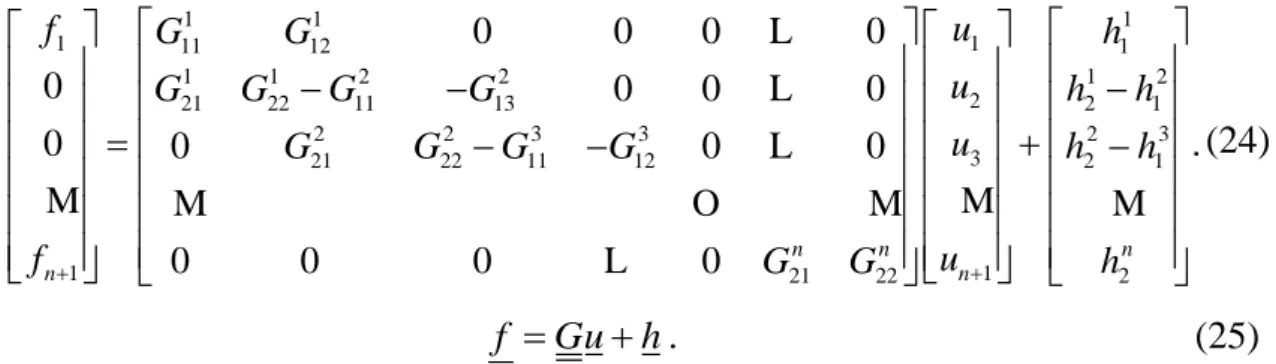
furthermore f₁ and f_n+1 are given. For the whole geometry the next system of equations can be derived for the displacement values u as basic variables :

1 1 1

1 11 12 1 1

1 1 2 2 1 2

21 22 11 13 2 2 1

2 2 3 3 2 3

21 22 11 12 3 2 1

1 21 22 1 2

0 0 0 0

0 0 0 0

0 0 0 0 .

0 0 0 0 ^{n n n}

n n

f G G u h

G G G G u h h

G G G G u h h

f _ G G u _ h

   

   

   

         

   

   

 

      

   

   

   

   

   

   

      

L L L

M M O M M M

L

(24)

f Guh. (25)

From Eqs. (24) and (25) the unknown displacement values (u_i, i=1...n+1) can be calculated, and then, using Eq. (21) the radial normal stresses can be evaluated.

4. NUMERICAL EXAMPLES

We consider a three-layered spherical component. The first and third layers are made of a thermal insulation material, while the material of the second one is steel.

For the numerical example the following data are used:

1 0.15m; 2 0.165m; 3 0.195m; 4 0.21m; 1 3 320GPa; 2 211GPa;

R  R  R  R  E E  E 

6

1 3 2 1 3 2 1 3

W W 1

0,21; 0,3; 4 ; 58 ; 7.4 10 ;

mK mK K

              ^

6

2 1 4

12 10 1; 20MPa; 0MPa; 523K; 273K.

K pⁱ p^o t t

   ^    

Figs. 3-7 indicate the results of this problem, solved with Maple 15, in three cases.

Figure 3. The temperature field

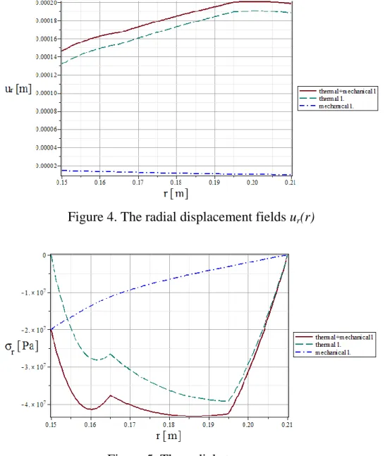
Figure 4. The radial displacement fields u_r(r)

Figure 5. The radial stresses σ_r

In Figs. 4-6 the red solid lines are the results of the thermomechanical problem with t₁=250ᴼC, p_i=20MPa, the blue dashdot lines indicate the results for the case when there is only mechanical loading (p_i=20MPa). The green dash lines illustrate the functions when there is only thermal loading (t₁=250ᴼC, p_i=0MPa)).

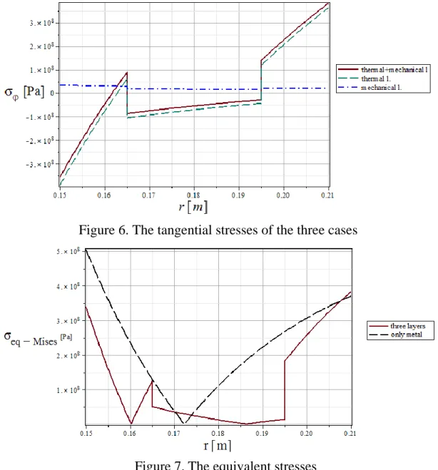
Fig. 7 indicates the von Mises equivalent stress of the thermomechanical problem (red solid line) and the black solid line is the curve for the case when all three layers are made of steel (the material of the middle layer in the original problem).

Figure 6. The tangential stresses of the three cases

Figure 7.The equivalent stresses

5. CONCLUSIONS

The main objective of this paper was to present an analytical solution for the displacement field and the associated stresses in hollow layered spherical bodies subjected to mechanical and thermal loads. To solve this problem the Fourier’s law of heat conduction and the exact solution for one layer were used, then the analytical solutions are derived via fitting the values of the displacement and stresses on the boundary surfaces of the layers. The developed solution can be utilized as Benchmark solutions for numerical methods to verify the accuracy of the considered numerical methods.

Acknowledgements: This research was supported by the European Union and the State of Hungary, co-financed by the European Social Fund in the framework of TÁMOP-4.2.4.A/ 2-11/1-2012-0001 ‘National Excellence Program’.

REFERENCES

[1] Carslaw, H. S., Jaeger, I. C.:Conduction of Heat in solids, Clarendon Press, Oxford, 1959.

[2] Boley, B. A., Weiner, J. H.: Theory of Thermal Stresses, John Wiley & Sons Inc., New York, 1960.

[3] Nowinski, I. L.: Theory of Thermoelasticity with Applications. Sythoff and Noordhoff, Alpen aan den Rijn, 1978.