3 4 5 6 7 8 9 10 11 12 13 14 15 16 17 18 19 20 21 22 23 24 25 26 27 28 29 30 31 32 33 34 35 36 37 38 39 40 41 42 43 44 45 46 47 48 49 50 51 52 53 54 55 56 57 58 59 60 61 62 63 64
Measuring expansion velocities in Type II-P supernovae
Q1
K. Tak´ats
1and J. Vink´o
1,2Q2
1Department of Optics and Quantum Electronics, University of Szeged, D´om t´er 9, Szeged, Hungary
2Department of Astronomy, University of Texas at Austin, Austin, TX 78712, USA
Accepted 2011 September 28. Received 2011 September 28; in original form 2011 March 28
A B S T R A C T
We estimate photospheric velocities of Type II-P supernovae (SNe) using model spectra
Q3 Q4
created withSYNOW, and compare the results with those obtained either by more conventionalQ5
techniques, such as cross-correlation, or by measuring the absorption minimum of P Cygni features.Based on a sample of 81 observed spectra of five SNe, we show thatSYNOWprovidesQ6
velocities that are similar to those obtained by more sophisticated non-local thermodynamic equilibrium modelling codes, but they can be derived in a less computation-intensive way.The estimated photospheric velocities (vmodel) are compared to those measured from Doppler shifts of the absorption minima of the Hβand the FeIIλ5169 features.
Our results confirm that FeIIvelocities (vFe) have a tighter and more homogeneous cor- relation with the estimated photospheric velocities than those measured from Hβ, but both suffer fromphase-dependent systematic deviations.The same is true for a comparison with
Q7
the cross-correlation velocities. We verify and improve the relations between vFe,vHβ and vmodel in order to provide useful formulae for interpolating/extrapolating the velocity curves of Type II-P SNe to phases not covered by observations. We also discuss implications of our results for the distance measurements of Type II-P SNe and show that the application of the model velocities is preferred in the expanding photosphere method.Key words: supernovae: general – supernovae: individual: SN 1999em – supernovae: indi- vidual: SN 2004dj – supernovae: individual: SN 2004et – supernovae: individual: SN 2005cs – supernovae: individual: SN 2006bp – distance scale.
Q8 Q9
1 I N T R O D U C T I O N
Type II-P supernovae (SNe) are core-collapse (CC) induced explo- sions that eject massive hydrogen-rich envelope. These SNe show a nearly constant-luminosity plateau in their light curve. The plateau phase lasts for∼100 d, and finally ends up in a rapid decline of the luminosity as the expanding ejecta become fully transparent.
CC SNe and their progenitors play important role in understand- ing the evolution of the most massive stars. Extensive searches for SN progenitors showed that the progenitors of Type II-P SNe are stars with initial masses between ∼8 and 17 M (Smartt et al.
2009). The lower value is roughly in agreement with the predic- tion of current theoretical evolutionary tracks, but the upper limit is somewhat lower than expected. The fate of the more massive (M≥ 20 M) stars is controversial. They are thought to be the input channel for Type Ib/c SNe (Gaskell et al. 1986), but this has not been confirmed directly by observations yet (Smartt 2009).
Any observational study of the physics of SNe and their progen- itors (and, obviously, all astronomical objects) depends heavily on E-mail: ktakats@titan.physx.u-szeged.hu (KT); vinko@titan.physx.u- szeged.hu (JV)
the knowledge of their distances. Because distance is such a crucial parameter, strong efforts have been devoted to the development of distance measurement techniques that are applicable for Type II-P SNe.
The expanding photosphere method (EPM) (Kirshner & Kwan 1974), a variant of the Baade–Wesselink method, uses the idea of comparing the angular and the physical diameter of the expanding SN ejecta. The input quantities are fluxes, temperatures and ve- locities observed at several epochs during the photospheric phase.
Thus, EPM requires both photometric and spectroscopic monitor- ing of SNe throughout the plateau phase. A clear advantage of EPM is that it does not require external calibration via SNe with known distances. Another interesting property is that EPM is much less sensitive to uncertainties in the interstellar reddening and absorp- tion towards SNe. As Eastman, Schmidt & Kirshner (1996, hereafter E96) have shown, 1-mag uncertainty inAV results in only∼8 per cent error in the derived distance. However, the assumption that the SN atmosphere radiates as a blackbody diluted by electron scatter- ing has raised some concerns. These led to the development of the applications of fullnon-local thermodynamic equilibrium (NLTE) model atmospheres, such as thePHOENIXcode in the spectral-fitting expanding atmosphere method (SEAM; Baron et al. 2004) or the
Q10
CMFGENcode by Dessart & Hillier (2005a,b). The drawback of these
C2011 The Authors
3 4 5 6 7 8 9 10 11 12 13 14 15 16 17 18 19 20 21 22 23 24 25 26 27 28 29 30 31 32 33 34 35 36 37 38 39 40 41 42 43 44 45 46 47 48 49 50 51 52 53 54 55 56 57 58 59 60 61 62 63 64
Table 1. Physical properties of the supernovae used in this paper.
SN t0 Distance cza E(B−V) MNi Mprog Referencesb
(JD 245 000) (Mpc) (km s−1) (mag) (10−2M) (M)
SN 1999em 1477.0 7.5–12.5 717 0.10 2.2 – 3.6 <15 1, 2, 3, 4, 5, 6, 7, 8
SN 2004dj 3187.0 3.2–3.6 131 0.07 1.3–2.2 12–20 9, 10, 11, 12, 13, 14, 15
SN 2004et 3270.5 4.7–6.0 48 0.41 5.6–6.8 9, 15–20 16, 17, 18, 19, 20, 21, 22
SN 2005cs 3549.0 7.1–8.9 463 0.05 0.3–0.8 6–13 23, 24, 25, 26, 27, 28, 29
SN 2006bp 3835.1 17.0–18.3 987 0.40 – 12–15 26, 30
aNED, http://nedwww.ipac.caltech.edu/
b References: (1) Hamuy et al. (2001); (2) Leonard et al. (2002); (3) Smartt et al. (2002); (4) Leonard et al. (2003); (5) Elmhamdi et al. (2003); (6) Baron et al. (2004); (7) Dessart & Hillier (2006); (8) Utrobin (2007); (9) Ma´ız-Apell´aniz et al.
(2004); (10) Kotak et al. (2005); (11) Wang et al. (2005); (12) Chugai et al. (2005); (13) Zhang et al. (2006); (14) Vink´o et al.
(2006); (15) Vink´o et al. (2009); (16) Li et al. (2005); (17) Sahu et al. (2006); (18) Misra et al. (2007); (19) Utrobin & Chugai (2009); (20) Poznanski et al. (2009); (21) Maguire et al. (2010b); (22) Crockett et al. (2011); (23) Maund, Smartt & Danziger (2005); (24) Pastorello et al. (2006); (25) Tak´ats & Vink´o (2006); (26) Dessart et al. (2008); (27) Eldridge, Mattila & Smartt (2007); (28) Utrobin & Chugai (2008); (29) Pastorello et al. (2009); (30)Immler et al. (2007).
Q11
approaches is that the building of tailored model atmospheres can be very time-consuming and needs much more computing power.
Also, in order to compute reliable models, the input observed spec- tra need to have sufficiently high signal-to-noise ratio(S/N) and spectral resolution.
Q12
The more recently developed standardized candle method (SCM;Hamuy & Pinto 2002;Hamuy 2003)relies on the empirical corre-
Q13
lation between the measured expansion velocity and the luminosity either in optical (Nugent et al. 2006; Poznanski et al. 2009) or in near-infrared (Maguire et al. 2010a) bands in the middle of the plateau phase,at+50 d after explosion.This method requires lessQ14
extensive input data, but needs a larger sample of Type II SNe with independently known distances in order to calibrate the empirical correlation. Because this is basically a photometric method which compares apparent and absolute magnitudes, SCM is more sensitive to interstellar reddening than EPM/SEAM, as mentioned above.Besides photometry, both EPM/SEAM and SCM need informa- tion on the expansion velocity at the photosphere (vphot). At first, EPM seems to be more challenging, because it requires multi-epoch observations, while SCM needs only the velocity at a certain epoch, at+50 d after explosion (v50). However, direct measurement ofv50
is possible only in the case of precise timing of the spectroscopic observation, which is rarely achievable.
The correct determination ofvphotis not trivial. As SNe expand homologously (v∼r, wherevis the velocity of a given layer and r is its distance from the centre), in most cases it is difficult to derive a unique velocity from the observed spectral features. The most frequently followed approach relies on measuring the Doppler shift of the absorption minimum of certain spectral features (mostly FeIIλ5169 or Hβ). Another possibility is the computation of the cross-correlation between the SN spectrum and a set of spectral tem- plates, consisting of either observed or model spectra, with known velocities. The third method is building a full NLTE model (such asPHOENIXorCMFGEN) for a given SN spectrum and adopting the theoreticalvphotfrom the best-fitting model.
The aim of this paper is to present a similar, but less computation- demanding approach to assign velocities to observed SN spectra.
We apply the simple parametrized codeSYNOW(Fisher 1999; Hatano et al. 1999) to model the observed spectra with an approximate, but self-consistent treatment of the formation of lines in the extended, homologously expanding SN atmosphere.To illustrate the appli-
Q15
cability ofSYNOW, we construct and fitted parametrized models to a sample of five well-observed, nearby Type II-P SNe that have a series of high-S/N spectra publicly available. We also check andre-calibrate some empirical correlations between velocities derived from various methods. The description of the observational sample is given in Section 2. In Section 3 we first review the different ve- locity measurement techniques for SNe II-P, and then we present the details of the application ofSYNOWmodels (Section 3.4). The results are collected and discussed in Sections 4 and 5, while the implications of the results for the distance measurements are given in Section 6. We draw our conclusions in Section 7.
2 DATA
Our sample contains 81 plateau phase spectra of five objects,SNe 1999em, 2004dj, 2004et, 2005cs and 2006bp.All five SNe are well- observed objects, they have been studied in detail and show a wide
Q16
variety in their physical properties (see Table 1).
SN 1999em was discovered on 1999 October 29 by Li (1999) in NGC 1637 at a very early phase. It is a very well-observed, well- studied object. The explosion date was determined as 245 1477.0± 2 JD (Hamuy et al. 2001; Leonard et al. 2002; Dessart & Hillier 2006). We used the spectra of Leonard et al. (2002) and Hamuy et al. (2001) downloaded from theSUSPECT1data base. Our sample contains 22 spectra, covering the first 80 d of the plateau phase.
SN 2004dj was discovered on 2004 July 31 by Itagaki (Nakano et al. 2004) in a young, massive cluster Sandage-96 of NGC 2403, about 1 month after explosion. We used the spectra taken by Vink´o et al. (2006). Due to the lack of observed spectrophotometric stan- dards, the flux calibration of those spectra was inferior, but this is not a major concern when only velocities are to be determined. We included 12 spectra taken between+47 and+100 d after explosion in our sample.
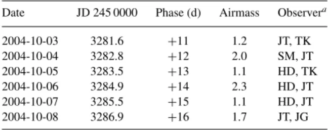
SN 2004et was discovered by Moretti (Zwitter, Murani & Moretti 2004) on 2004 September 27 in NGC 6946. The spectra of Sahu et al.
(2006) (downloaded fromSUSPECT) and Maguire et al. (2010b) were used, together with six previously unpublished early-phase spectra taken with the 1.88-m telescope at the David Dunlap Ob- servatory (DDO;see Appendix A). The 22 spectra cover the period
of+11 to+104 d after explosion.
Q17
SN 2005cs was discovered on 2005 June 29 by Kloehr et al.
(2005) in M51. Due to its very early discovery and proximity, this object is very well sampled and studied in detail. It is an underlumi- nous, low-energy, Ni-poor SN that had a low-mass progenitor (see
1Available from http://suspect.nhn.ou.edu/∼suspect/
C2011 The Authors
3 4 5 6 7 8 9 10 11 12 13 14 15 16 17 18 19 20 21 22 23 24 25 26 27 28 29 30 31 32 33 34 35 36 37 38 39 40 41 42 43 44 45 46 47 48 49 50 51 52 53 54 55 56 57 58 59 60 61 62 63 64
Table 1 for references). 14 spectra of Pastorello et al. (2006, 2009) were used, which were obtained between days+3 and+61.
SN 2006bp was discovered on 9th April 2006 by Nakano &
Itagaki (2006) in NGC 3953, also in a very early phase. We used 11 spectra of Quimby et al. (2007), downloaded fromSUSPECT, covering the period between+5 and+72 d.
3 T H E I S S U E O F M E A S U R I N G E X PA N S I O N V E L O C I T I E S I N S N e
During the photospheric phase, the homologously expanding Type II-P SN ejecta consist of two parts: the outer, partly transparent atmosphere where the observable spectral features are formed, and an optically thick inner part, which emits most of the continuum radiation as a ‘diluted’ blackbody (e.g. E96). Because the inner part is mostly ionized, the major source of the total opacity is electron scattering. Thus, theinstantaneousphotosphere is located at the depth where the outgoing photons are last scattered, i.e. where the electron-scattering optical depth isτe∼2/3 (Dessart & Hillier 2005a, hereafter D05). This is presumed to occur in a thin, spherical shell at a certain radiusrphot, and the homologous expansion gives this a unique velocityvphot=vrefrphot/rref, whererrefis the radius of an (arbitrary) reference layer andvrefis its expansion velocity.
As the ejecta expand and dilute, the photosphere migrates inwards, towards the inner layers of the ejecta that expand at a slower rate;
thusvphotcontinuously declines with time.
Q18
The issue of measuringvphotcomes from the fact that no mea- surable spectral feature is connected directly tovphot. As previously mentioned in Section 1, there exist several observational/theoretical approaches toestimatevphotfrom observed spectra. In the follow- ing, we briefly review these methods, summarizing their advan- tages/drawbacks.3.1 P Cygni lines
The most widely used method is to measure the velocity represented by the minimum flux of the absorption component of an unblended P Cygni line profile (sometimes referred to as ‘maximum absorption’, vabs; Dessart & Hillier 2005b). This is motivated by the theory of P Cygni line formation (e.g. Kasen et al. 2002), which predicts that the minimum flux in a P Cygni line occurs at the velocity of the photosphere. Strictly speaking, this is only true for an optically thin line formed by pure scattering. In most cases, the FeIIλ5169 feature is used for measuring vabs, for which Dessart & Hillier (2005b) pointed out that it can represent the truevphotwithin 5–10 per cent accuracy. However, Leonard et al. (2002) showed that using weaker, unblended features one can get∼10 per cent lower velocities than from the FeIIλ5169 feature. This raises the question of whether the measurable lines were indeed optically thin and unblended, and which one represented the true vphot. Moreover, Dessart &
Hillier (2005b) also revealed thatvabs can either overestimate or underestimatevphot, depending on various physical conditions, such as the density gradient and the excitation/ionization conditions for the particular transition within the ejecta.
While the FeIIλ5169 feature can be relatively easily identified and measured in Type II-P SNe spectra obtained later than∼20 d after explosion (which is undoubtedly a major advantage of this method), this is not so for earlier phases. In early-phase spectra only the Balmer lines and maybe HeIfeatures (mostly theλ5876 feature) can be identified. These features are less useful for mea- suringvphot, because none of them is optically thin and the HeI
λ5876 feature can sometimes be blended with NaID. Moreover,
their line profile shapes often make the location of the minimum of absorption component difficult to determine (Dessart & Hillier 2005b, 2006).
Also, in spectra having less S/N, the weaker FeIIfeatures are often buried in the noise, making them inappropriate for veloc- ity measurement. In these cases, several authors attempted to use the stronger features, especially Hβ. Although Dessart & Hillier (2005b) pointed out thatvHβ is certainly less tightly connected to vphotthan the weaker FeIIλ5169 feature, Nugent et al. (2006) have shown that the ratiovHβ/vFe is∼1.4 below vHβ = 6000 km s−1 and linearly decreases for higher velocities. Recently, this corre- lation was revised by Poznanski, Nugent & Filippenko (2010) by revealing an entirely linear relation betweenvHβ andvFe, but re- stricting the analysis only to velocities measured between+5 and +40 d after explosion. The uncertainty of estimatingvFefromvHβ
is∼300 km s−1(Poznanski et al. 2010). It is emphasized that these empirical relations are more or less valid between the velocities of two observable features, but both of them may be systematically off from the truevphot. Indeed, Dessart & Hillier (2005b) found thatvHβ
can be either higher or lower thanvphotwith an overall scattering of±15 per cent. For velocities below 10 000 km s−1vHβis usually higher thanvphot, in accord with the empirical correlations withvFe, but above 10 000 km s−1it can be lower thanvphot.
3.2 Cross-correlation
Motivated by the uncertainties of measuring the Doppler shift of a single, weak feature in a noisy spectrum, several authors proposed the usage of the cross-correlation technique, which is a powerful method for measuring Doppler shifts of stellar spectra containing many narrow spectral features. This method predicts the Doppler shift of theentirespectrum by computing the cross-correlation func- tion (CCF) between the observed spectrum and a template spec- trum with a priori known velocityvtempl. The resulting velocity is vcc=vrel+vtempl, wherevrelis the velocity at which the CCF reaches its maximum (i.e. the relative Doppler shift between the observed spectrum and the template).
However, the applicability of cross-correlation for SN spectra is not obvious, because of the physics of P Cygni line formation in SN atmospheres. Ifvphotis higher, then the centre of the absorp- tion component gets blueshifted, while the centre of the emission component stays close to zero velocity. Thus, cross-correlating two spectra with differentvphot, the relative velocity will underestimate the true velocity difference between the two spectra. This is illus- trated in Fig. 1, where we determined the CCF between two Type II-P SN model spectra (computed withSYNOW, see below) that were identical except theirvphotwhich differed byvphot=2000 km s−1. The cross-correlation was computed only in the 4500–5500 Åin- terval to exclude the Hαfeature. This was done for an early-phase spectrum containing only H and He features (Fig. 1, left panel) and a later-phase spectrum with more developed metallic lines (Fig. 1, right panel). It is visible in the bottom panels that the maximum of the CCF (i.e.vrel) is shifted towards lower velocities with respect to the truevphot(indicated by a dotted vertical line in the CCF plot) for both spectra. The systematic offset ofvrelfrom vphotis∼200 km s−1 for the later-phase spectrum that contains many narrower absorption features, and it reaches ∼700 km s−1 for the early-phase spectrum that is dominated by broad Balmer lines with a stronger emission component. These simple tests are in very good agreement with the results of Hamuy et al. (2001) and Hamuy (2002), who applied the cross-correlation technique us- ing model spectra of E96 with a-priori knownvphot as templates.
C2011 The Authors
3 4 5 6 7 8 9 10 11 12 13 14 15 16 17 18 19 20 21 22 23 24 25 26 27 28 29 30 31 32 33 34 35 36 37 38 39 40 41 42 43 44 45 46 47 48 49 50 51 52 53 54 55 56 57 58 59 60 61 62 63 64
0 0.1 0.2 0.3 0.4 0.5 0.6 0.7 0.8 0.9 1
4000 5000 6000 7000
Flux
Wavelength (Å) Model +8 d
0 0.05 0.1 0.15 0.2 0.25 0.3 0.35 0.4
4000 5000 6000 7000 Wavelength (Å)
Model +41 d
0.2 0.3 0.4 0.5 0.6 0.7 0.8 0.9 1
0 2000 4000
Correlation function
Velocity (km/s) Model +8 d
0 0.2 0.4 0.6 0.8 1
0 2000 4000 Velocity (km/s)
Model +41 d
Figure 1. Model spectra of a Type II-P SN in the early-phase (top left) and late-phase (top right), and the resulting CCFs (bottom panels) after cross-correlating
Q19
the spectra with their identical models but having a 2000 km s−1highervphot. The arrows mark the peak location of the CCFs, while the true relative velocity differencevphotis indicated by the dotted vertical line. The peak of the CCF underestimatesvphotin both cases.They pointed out that vrel usually underestimates vphot so that vphot/vrel∼1.18, with the scatter of∼900 km s−1.
Another variant of the CCF method was proposed by Poznanski et al. (2009), and was also applied by D’Andrea et al. (2010) and Poznanski et al. (2010). They took their template spectra from the li- brary of the SuperNova IDentification codeSNID2(Blondin & Tonry 2007) that contains high-S/N observed spectra of many SNe, but used only those templates that showed a well-developed FeIIλ5169 feature. The reason for their choice was that they wanted to esti- matevFeat+50 d after explosion (v50), which is an input parameter in SCM. This template selection caused the well-known issue of template mismatch that further biases the cross-correlation results.
As D’Andrea et al. (2010) concluded, this template mismatch can result in significant underestimate ofvFeby∼1500 km s−1for spec- tra obtained att<20 d, and is also present in later-phase spectra, although it is less pronounced,∼300–400 km s−1. To overcome this problem, in a subsequent paper Poznanski et al. (2010) suggested the application of theirvFeversusvHβ relation to estimatevFeby measuringvHβ for these early-phase spectra and then propagate the resulting velocity to day +50. Nevertheless, the two groups presented velocities that were different by 200 to 1000 km s−1for the same set of SNe spectra fromthe SDSS-II survey.This under-
Q20
lines that although cross-correlation seems to be an easy and robust method that gives reasonable velocities even for low-S/N spectra, the results may be heavily biased, especially at early phases, when the SN spectra contain only a few, broad features.3.3 Tailored modelling
Tailored modelling of the whole observed spectrum via NLTE mod- els was invoked e.g. by Baron et al. (2004) using the codePHOENIX,
2Available from http://marwww.in2p3.fr/∼blondin/software/snid/index.
html
and Dessart & Hillier (2006) and Dessart et al. (2008) with the code
CMFGEN. Here,vphotis determined implicitly by requiring an overall fit of the entire observed spectrum by a synthetic spectrum from a full NLTE radiation-hydrodynamic model. In these models the location of the photosphere is usually defined as the layer where the electron scattering optical depth reaches unity or 2/3 (e.g. D05).
vphotis then simply determined by the radiusrphotand the law of homologous expansion (see above). Although this is probably the best self-consistent method for obtaining SN velocities, building full NLTE models for multiple epochs requires a large amount of computing power. Thus, its usage for a larger sample of SNe would be very time-consuming and impractical. Also, in some cases a good global fit to the whole spectrum may not be equally good for individual spectral lines, where a large number of physical details play important role in the formation of the given features. This may lead to some uncertainties in the velocities given by the models, which will be illustrated in Section 4.
3.4 Using synow
The success of tailored spectrum models to estimatevphot sug- gests a similar, but much more simplified approach: the usage of parametrizedspectrum models that do not contain the computation- intensive details of NLTE level populations or exact radiative trans- fer calculations, but preserve the basic physical assumptions of an expanding SN atmosphere, and able to reproduce the formation of P Cygni lines in a simplified manner. Such models can be com- puted either with theSYNOWcode (Branch et al. 2002) or using the more recently developedSYNAPPScode (Thomas, Nugent & Meza 2011) that has a parameter-optimizer routine built-in. In this paper we applySYNOWto calculate model spectra. BecauseSYNOWdoes only spectrum synthesis and has no fitting capabilities, we used self-developed UNIX shell scripts to fine-tune the parameters until a satisfactory fit to the observed spectrum is achieved.
C2011 The Authors
3 4 5 6 7 8 9 10 11 12 13 14 15 16 17 18 19 20 21 22 23 24 25 26 27 28 29 30 31 32 33 34 35 36 37 38 39 40 41 42 43 44 45 46 47 48 49 50 51 52 53 54 55 56 57 58 59 60 61 62 63 64
4000 4500 5000 5500 6000 6500 7000
Scaled flux
4700 4900
4000 4500 5000 5500 6000 6500 7000 5100 5200
Wavelength (Angstroms)
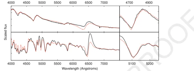
Figure 2. The observed (black solid line) and best-fitting model (red dashed line) spectra of SN 1999em on days+9 (top) and+41 (bottom). The right panels enlarge the wavelength regions of the fitted lines: Hβ(top) and FeIIλ5169 (bottom).
The basic assumptions ofSYNOWare the followings: (i) the SN ejecta expand homologously; (ii) the photosphere radiates as a blackbody; (iii) spectral lines are formed entirely above the photo- sphere; (iv) the line formation is due to pure resonant scattering.
Level populations are treated in LTE and the radiative transfer equa- tion is solved in the Sobolev approximation (see also e.g. Kasen et al.
2002).
When running SYNOW, several parameters must be set. These are the temperature of the blackbody radiation (Tbb) emitted by the photosphere, the expansion velocity at the photosphere (vphot), the chemical composition of the ejecta and the optical depth of a reference line (τref) of each compound. For each atom/ion, the optical depths for the rest of the lines are calculated assuming Boltzmann excitation governed by the excitation temperatureTexc. The location of the line-forming region in the atmosphere can be tuned for each compound by setting the velocities of the lower and upper boundary layers,vminandvmax. The optical depth as a function of velocity (i.e. radius) can be modelled either as a power law or as an exponential function. We assumed power-law atmospheres and adjusted the power-law exponentnto reach optimal fitting.
After setting the initial values by hand, several models in a wide range ofvphot,nandτrefwere created for a pre-selected set of ions.
In order to reduce the number of free parameters, we initially set Tbb (which has very little effect on the line shapes) to represent the continuum of the fitted spectrum and kept it fixed during the optimization. Moreover, we applied a single power-law exponent nfor all atoms/ions. We also assumed that all spectral features are photospheric, thus fixingvminwell below the photosphere andvmax
at∼40 000 km s−1.
The best-fitting model was then chosen viaχ2-minimization, and the fitting process was iterated for a few times, each time resampling the parameter grid in the vicinity of the minimum of theχ2function found in the previous iteration cycle. This way we determined the parameters and the chemical compositions that best describe the observed spectra.
Then, to further refine the estimated photospheric velocity, we fine-tuned onlyvphotof the best-fitting model and calculated theχ2 function only in the vicinity of certain lines instead of the whole spectrum. This may reduce the systematic underestimate or over- estimate ofvphotproduced by false positive fitting to the observed spectrum outside the range of the spectral features considered.
Motivated by the results of Dessart & Hillier (2005b) (see Section 3.1), we have chosen the FeIIλ5169 feature for this fine- tuning process. When this feature was not present in the observed spectrum (i.e. the early-phase spectra, before∼15 d), we used Hβ (see Section 3.1) instead. Hereafter we denote thevphotparameter of the best-fittingSYNOWmodel asvmodel. Errors ofvmodelwere es- timated by choosing the 90 per cent confidence interval around the minimum of theχ2function.
Fig. 2 shows two examples for an early- and a later-phase spec- trum of SN 1999em together with the best-fitting model. The right- hand panel zooms in on the region of Hβand FeII λ5169. Note that although the final fitting was restricted to the proximity of these lines, the best model describes the entire observed spectrum (except Hα) very well.
This velocity measurement method has multiple sources of error.
One of them may be the systematic bias due to the approximations in the model (LTE, power-law atmosphere, simple source function etc.). However, the comparison of our results with those from full NLTECMFGENmodels (Section 4) shows no systematic bias in the case of SNe 1999em and 2005cs. The agreement between the ve- locities from these two very different modelling codes is within
±10 per cent. For SN 2006bp, the differences are higher, but it will be shown below that for this SN theCMFGENmodels do not describe well the spectral features we use, in contrast to theSYNOWmodels (Section 4.5).
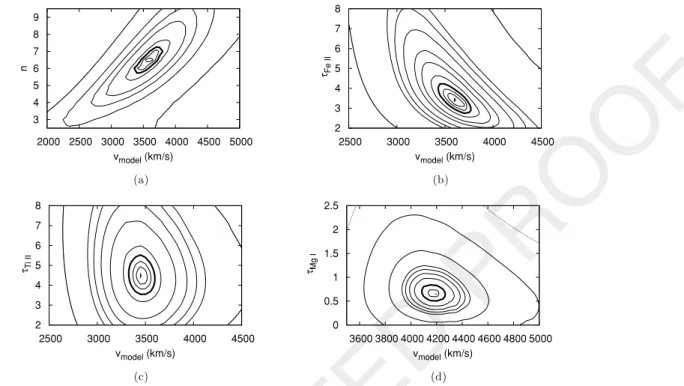
Another source of error may be the correlation between the pa- rameters. In Fig. 3 we present contour plots of theχ2hyperspace around its minimum, as a function ofvmodel and several other pa- rameters that can affect the shape of the fitted FeIIλ5169 feature.
The thick black contour curve corresponds to 50 per cent higher χ2than the minimum value. It is visible that the correlation is in- deed present (i.e. the contours are distorted) betweenvmodeland the power-law exponentnor the optical depthτFe. The correlation is much less betweenvmodelandτrefof TiIIand MgI, whose features may blend with FeIIλ5169. However, even for the correlated pa- rameters, selectingnorτFevery far from their optimum value can altervmodelonly by a few hundred km s−1. Thus, we conclude that uncertainties in finding the minimum ofχ2do not cause errors in vmodelthat significantly exceed the uncertainty due to the spectral resolution of the observed spectra (which is usually between 200 and 300 km s−1).
C2011 The Authors
3 4 5 6 7 8 9 10 11 12 13 14 15 16 17 18 19 20 21 22 23 24 25 26 27 28 29 30 31 32 33 34 35 36 37 38 39 40 41 42 43 44 45 46 47 48 49 50 51 52 53 54 55 56 57 58 59 60 61 62 63 64
2000 2500 3000 3500 4000 4500 5000 vmodel (km/s)
3 4 5 6 7 8 9
n
2500 3000 3500 4000 4500 vmodel (km/s)
2 3 4 5 6 7 8
τFe II
2500 3000 3500 4000 4500 vmodel (km/s)
2 3 4 5 6 7 8
τTi II
3600 3800 4000 4200 4400 4600 4800 5000 vmodel (km/s)
0 0.5 1 1.5 2 2.5
τMg I
Figure 3. Contour plot of theχ2function around its minimum, as a function ofvmodeland power-law exponentn(a),τrefof FeII(b), TiII(c) and MgI(d).
The thick black contour curve corresponds to 50 per cent higherχ2than the minimum value. The parameters plotted in (a) and (b) are definitely correlated, while the correlation is much less between the parameters in (c) and (d).
A possible source of uncertainty may be that during the final fitting the wavelength interval around the used spectral feature is chosen somewhat subjectively. However, our tests showed that changing the limits reasonably has a negligible effect on the final velocities.
It is emphasized that although the final fitting is restricted to the vicinity of a well-defined spectral line, this method is certainly more reliable than the measurement of only the location of the minimumof the same feature. As discussed above, the minimum can be significantly and systematically altered by S/N, spectral resolution, blending etc. The fitting of a model spectrum to the entirefeature is expected to overcome these difficulties, provided the underlying model is not too far from reality.
4 C O M PA R I N G T H E R E S U LT S F R O M D I F F E R E N T M E T H O D S
Using SYNOWas described above, we determined the best-fitting parameters of all SNe spectra from Section 2. The resulting model velocities are collected in Table B1 in Appendix B. The best-fitting
SYNOWparameters, such asτref for each atom/ion, the power-law exponentnandvmodeltogether with the chosenTphot, can be found in Table C1 in Appendix C. In Table B1 we also list thevFeandvHβ
velocities. For SNe 1999em, 2005cs and 2006bp, we collected the photospheric velocities fromCMFGENmodels of Dessart & Hillier (2006) and Dessart et al. (2008). These are included in Table B1 as vnlte. Velocities from the cross-correlation technique (Section 3.2) were obtained using two sets of template spectra. The first set contained the 22 observed spectra of SN 1999em (set 1), while the second set was based on theCMFGENmodels mentioned above (set 2). The velocities of the template spectra werevFefor set 1 and vnltefor set 2. We cross-correlated all the observed spectra with the two sets separately on the wavelength range of 4500–5500 Å, and the resulting velocities are also given in Table B1 asvcc.
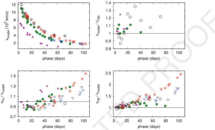
Fig. 4 showsvmodel against phase for all studied SNe (top left panel) and the ratio ofvmodel to all the other velocities. The cal- culated velocities all show the expected decline with phase as the photosphere moves much deeper within the ejecta,towards slower expanding layers.
Similar plots containing the ratiovmodel/vccandvabs/vccas func-
Q21
tions of phase are presented in Fig. 5.
In the following, we provide some details of deriving these ve- locities for each object and discuss some object-specific differences between them.
4.1 SN 1999em
When determiningvmodel withSYNOW, Hβ was fitted for the first six spectra, then the FeIIλ5169 feature was used for the remain- ing 16 spectra. The resulting velocities are between 11 000 and 1800 km s−1. As seen in the bottom right panel of Fig. 4,vmodeland vHβare about the same for the early phases (before the appearance of the FeIIlines), while latervHβ tends to be higher thanvmodel. Also, between day+15 and day+40,vmodelis slightly higher than vFe(Fig. 4, bottom left panel). After day+40,vmodel drops below vFeand their ratio increases towards later phases.
The velocities fromCMFGENmodels of Dessart & Hillier (2006) (Fig. 4, top right panel) agree withvmodel. The cross-correlation with set 2 (Fig. 5, bottom panels) gave similar results for the first few points, but overestimatevmodel between days+22 and+80.
They mostly fall betweenvHβandvFe, which is expected, since we cross-correlated the range of 4500–5500 Å, where these features appear.
4.2 SN 2004dj
TheSYNOWmodel velocities of the 11 spectra that cover the second half of the plateau phase are between∼3400 and 1700 km s−1. These
C2011 The Authors
3 4 5 6 7 8 9 10 11 12 13 14 15 16 17 18 19 20 21 22 23 24 25 26 27 28 29 30 31 32 33 34 35 36 37 38 39 40 41 42 43 44 45 46 47 48 49 50 51 52 53 54 55 56 57 58 59 60 61 62 63 64
2 4 6 8 10 12
0 20 40 60 80 100
vmodel (103 km/s)
phase (days)
0.8 0.9 1 1.1 1.2 1.3 1.4
0 20 40 60 80 100
vmodel / vnlte
phase (days)
0.7 0.9 1.1 1.3 1.5
0 20 40 60 80 100
vFe / vmodel
phase (days)
1 1.5 2 2.5
0 20 40 60 80 100
vHβ / vmodel
phase (days)
Figure 4. Top left: model velocities (vmodel) fromSYNOWas functions of phase. Top right: the ratio ofSYNOWandCMFGENmodel velocities (vmodel/vnlte) against phase. Bottom panels: the phase dependence ofvFe/vmodel(bottom left) andvHβ/vmodel(bottom right). Symbols represent the following: filled circles, SN 1999em; open circles, SN 2006bp; filled triangles, SN 2005cs; open triangles, SN 2004dj; asterisks, SN 2004et.
0.6 0.7 0.8 0.9 1 1.1 1.2 1.3
0 20 40 60 80 100
vmodel / vcc#1
phase (days)
0.6 0.7 0.8 0.9 1 1.1 1.2 1.3
0 20 40 60 80 100
vabs / vcc#1
phase (days)
0.6 0.8 1 1.2 1.4
0 20 40 60 80 100
vmodel / vcc#2
phase (days)
0.6 0.8 1 1.2 1.4
0 20 40 60 80 100
vabs / vcc#2
phase (days)
Figure 5. Top panels: ratio ofvmodelandvabstovccfrom cross-correlating with the observed spectra of SN 1999em (set 1, see text) as functions of phase.
Bottom panels: the same as above, but with respect to the template set containingCMFGENmodels (set 2). The symbols represent the same SNe as in Fig. 4.
C2011 The Authors
3 4 5 6 7 8 9 10 11 12 13 14 15 16 17 18 19 20 21 22 23 24 25 26 27 28 29 30 31 32 33 34 35 36 37 38 39 40 41 42 43 44 45 46 47 48 49 50 51 52 53 54 55 56 57 58 59 60 61 62 63 64
4000 5000 6000 7000 8000 9000
Scaled flux
Rest wavelength (Angstrom)
4600 4800 5000 5200 5400
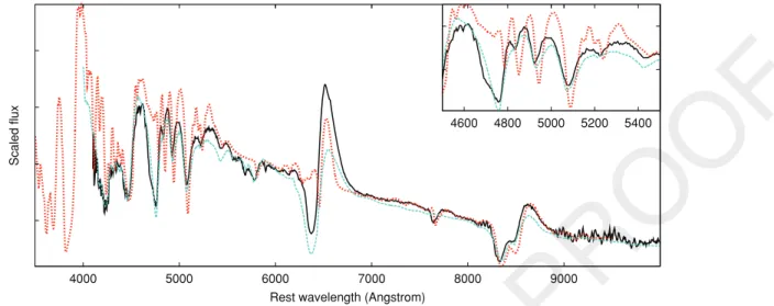
Figure 6. Plot of theCMFGEN(red dotted line) and theSYNOWmodels (turquoise dashed line) and the observed spectra (black continuous line) of SN 2006bp on day+32 (see text).
are similar to those of SN 1999em at the same phase. BothvFeand vHβare higher thanvmodelat all epochs, especially the latter with a factor of about 1.8 (Fig. 4).
NoCMFGENmodel was available for SN 2004dj. Cross-correlation with both template sets gave very similar results. They are only slightly higher than bothvmodelandvFe(Fig. 5).
4.3 SN 2004et
For the first six spectra, theSYNOWmodel was optimized for Hβ, then for the FeIIλ5169 feature. The resulting model velocities are between 9700 and 1800 km s−1(Fig. 4). ThevFevalues are similar tovmodel, but their ratio shows a slight phase dependence, similar to the other SNe studied here. In contrast, the values ofvHβ are very different fromvmodel. At early phases, they are close tovmodel
(except for the first point), but later thevHβtovmodelratio strongly increases, reaching as high as 2.5.
Again, there is noCMFGENmodel available for this SN. Cross- correlation with set 1 resulted in velocities similar tovHβ at early phases and tovFelater. With set 2, cross-correlation gave similar results at early phases, but later it produced systematically higher ve- locities. This underlines the importance of selecting proper template spectra and template velocities when applying the cross-correlation technique.
4.4 SN 2005cs
We used the Hβline for fitting the first three spectra withSYNOW. The velocities of this SN are very low: they are in the range of 7100–
1100 km s−1and decrease quickly. The velocities from absorption minima are very close tovmodelfor both Hβand FeIIλ5169. ThevFe
values follow the tendency similar to the previous objects: they are somewhat lower thanvmodelat the early phases, but become higher after about day+30. ThevHβvalues are much closer tovmodelthan for the other SNe, and thevHβ/vmodel ratio stays about the same for all epochs (Fig. 4). The velocities of theCMFGEN models for SN 2005cs are the same as thevmodelvalues for all epochs, except for day+9. Cross-correlation with both template sets resulted in velocities close tovFe.
4.5 SN 2006bp
The results for SN 2006bp are controversial. ApplyingSYNOW, the Hβline was fitted for the first 4 of the 11 observed spectra, while FeIIλ5169 was used for the rest. The model velocities are between 12000 and 3800 km s−1. BothvFe and vHβ follow the tendency shown by other SNe (Fig. 4).
In contrast, unlike in the previous two cases, the velocities from theCMFGENmodels differ significantly from ourvmodel values. At early epochs, this difference is much lower (∼500–700 km s−1), being close to zero at day+15. After day+15, it becomes higher reaching∼1200 km s−1on day+32. At later phases, the difference decreases somewhat, but stays being significant.
Cross-correlating the same spectra with theCMFGENmodels using the wavelength range of 4500–5500 Å resulted in velocities that are very close tovmodel(except for day+9). Using the first template set, the results agree well withvFe, orvHβat early epochs.
To examine the obvious controversy between the velocity of the
CMFGENmodels and that of all the others, we plotted the observed spectra and the best-fittingCMFGENmodel on day+32 (when the differences are the highest) in Fig. 6. Zooming in on the range of 4500–5500 Å clearly shows that the model by Dessart et al. (2008) does not fit these spectral features well, leading to an underestimate of the velocity. Thus, we suspect that the velocity differences we found are probably due to the inferior fitting of theCMFGENmodels to the SN 2006bp spectra.
5 D I S C U S S I O N
As shown in the previous sections, the photospheric velocities of four SNe in our sample evolved similarly. SNe 1999em, 2004et and 2006bp had high velocities at early phases and they decreased quickly, although their decline slopes were different. SN 2004dj probably showed similar evolution, but the lack of the early-phase data prevents a more detailed comparison. In contrast, SN 2005cs was a very different, low-energy SN II-P as discussed in detail in previous studies. It had lower early velocities and the velocity curve decreased much faster than for all the other SNe.
As expected, the different velocity measurement methods we applied provided somewhat different results. As seen in Fig. 5, the velocities obtained from cross-correlation are usually closer to
C2011 The Authors
3 4 5 6 7 8 9 10 11 12 13 14 15 16 17 18 19 20 21 22 23 24 25 26 27 28 29 30 31 32 33 34 35 36 37 38 39 40 41 42 43 44 45 46 47 48 49 50 51 52 53 54 55 56 57 58 59 60 61 62 63 64
0.7 0.8 0.9 1 1.1 1.2 1.3 1.4 1.5 1.6
0 2000 4000 6000 8000 10000
vFe / vmodel
vmodel (km/s)
1 1.5 2 2.5
0 2000 4000 6000 8000 10000 12000 vHβ / vmodel
vmodel (km/s)
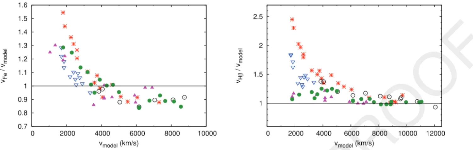
Figure 7. ThevFe/vmodel(left-hand panel) andvHβ/vmodel(right-right panel) ratio against the model velocities. The symbols have the same meaning as in Fig. 4.
vabs than tovmodel. This is understandable, given that the cross- correlation method is most sensitive to the shapes and positions of the spectral features that may be biased towards lower or higher ve- locities. Thevmodel/vccratio (Fig. 5, top left and bottom left panels) shows the same trend (but plotted upside down) as thevFe/vmodel
ratio in Fig. 4 (bottom left panel), i.e. vmodel is higher between days 10 and 50, but becoming smaller thanvFeorvcc. On the other hand, no such systematic trend can be identified between vmodel
andvnlte(Fig. 4, top right panel). These benchmarks suggest that the model velocities, either fromSYNOWor fromCMFGEN, are consis- tent, and show phase-dependent offsets from the absorption minima or cross-correlation velocities. The increasing systematic offset is particularly strong forvHβ (Fig. 4, bottom right panel). Thus, the traditional, simple measurement methods seem to underestimate the true photospheric velocities before day 50, but increasingly overes- timate them towards later epochs. This should be kept in mind when the true photospheric velocities are needed, e.g. in the application of EPM.
In order to do further testing, we plotted the ratio ofvFe/vmodel
andvHβ/vmodelas a function ofvmodelfor all SNe, following Dessart
& Hillier (2005b) (Fig. 7). The vFe/vmodel ratio shows the same trend for all objects: at high velocities (i.e. early phases) the ratio is somewhat lower than 1, then it reaches unity around∼4000 km s−1, and below that it keeps rising, reaching∼ 1.6 by the end of the plateau. ThevHβ/vmodel ratio is more complicated. At highvmodel
values, it is around 1, but becomes higher than unity aroundvmodel≈ 7000 km s−1. Below that the slope of the rising changes from object to object. In the case of SNe 2005cs and 1999em, this ratio stays under∼1.4, while for the other three SNe it becomes much higher.
For SN 2006bp, there are no spectra belowvmodel =3850 km s−1, but above that its evolution seems to be similar to that of SN 2004et.
A similar plot was published by Dessart & Hillier (2005b) based on their set ofCMFGENmodel spectra (see their fig. 14). The only slight difference is that they plotted the ratio of the velocity mea- sured from the absorption minima of the model spectra to the input velocity of the code, as a function of the input velocities. Although they did not have data below∼4000 km s−1, and we do not have data above∼12 050 km s−1, between these limits their plotted values are mostly similar to ours. In their fig. 14, the FeIIλ5169 velocities are lower than that of the model for high velocities, and their ratio reaches 1 between 5000 and 4000 km s−1, just like our data. The situation is somewhat different for Hβ. At high velocities the two results are consistent: above∼11 000 km s−1, the data by Dessart
& Hillier (2005b), as well as ours, are around 1. However, their velocity ratio exceeds 1 at∼8000 km s−1 and has a highest value of 1.15 for Hβ. It is much lower than our results in Fig. 7. In the case of SN 2004et, our velocity ratio goes as high as 2.5. It must be noted, however, that the model spectra used by Dessart &
Hillier (2005b) were tailored to represent SNe 1987A and 1999em (D05). The latter object is also in our sample, and ourvHβtovmodel
ratio for that particular SN is similar to the results of Dessart &
Hillier (2005b). Thus, it is probable that the lowervHβ/vmodelratio of Dessart & Hillier (2005b) is due to the limited parameter range of theirCMFGENmodels used to create their plot.
Recently, Roy et al. (2011) published a study of velocity measure- ment for the Type II-P SN 2008gz. They applied a similar technique of usingSYNOWto fit FeIIfeatures around 5000 Å. They also esti- mated the velocity from the absorption minima of these lines. They obtained 4200±400 km s−1and 4000±300 km s−1forvmodeland vFe, respectively, from a+87-d spectrum. This result is consistent with our findings plotted in Fig. 7:vFeis practically equal tovmodel
around 4000 km s−1.
5.1 Velocity–velocity relations
Using the synthetic spectra of E96 and D05, Jones et al. (2009) also examined the relation betweenvHβandvmodel. They found that their ratio can be described as
vHβ
vmodel
= 2
j=0
ajvHjβ, (1)
where the values ofajare given in Table 2. In Fig. 8(a) we plotted our data together with these polynomials. The polynomials based on the D05 models overestimate ourvmodelvalues (rmsσ=0.412), Table 2.Polynomial coefficients for the vHβ and vFe to vmodel ratio (equation 1).
j 0 1 2 σ References
aj(Hβ) (E96) 1.775 −1.435e–4 6.523e–9 0.30 1 aj(Hβ) (D05) 1.014 4.764e–6 −7.015e–10 0.41 1 aj(Hβ) 1.528 −1.551e–5 −3.462e–9 0.27 2 aj(Hβ) without 04et 1.578 −8.573e–5 3.017e–9 0.17 2 aj(FeIIλ5169) 1.641 −2.297e–4 1.751e–8 0.11 2 References.(1) Jones et al. (2009); (2) this paper.
C2011 The Authors
3 4 5 6 7 8 9 10 11 12 13 14 15 16 17 18 19 20 21 22 23 24 25 26 27 28 29 30 31 32 33 34 35 36 37 38 39 40 41 42 43 44 45 46 47 48 49 50 51 52 53 54 55 56 57 58 59 60 61 62 63 64
2000 4000 6000 8000 10000 12000
2000 4000 6000 8000 10000 12000 vmodel (km/s)
vHβ (km/s) E96
D05 with 2004et w/o 2004et
1000 2000 3000 4000 5000 6000 7000 8000
1000 2000 3000 4000 5000 6000 7000 8000 vmodel (km/s)
vFe (km/s)
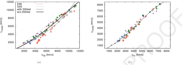
Figure 8. (a) The plot ofvmodelagainstvHβ. The lines represent the polynomials calculated by Jones et al. (2009) (see text) based on the models of E96 (red dotted line) and D05 (blue dashed line). The result from our fitting on all SNe is plotted as a black dotted line while the fitting that omits SN 2004et is shown by a black solid line. (b) The same fitting as (a) but forvFeusing all SNe. The symbols have the same meaning as in Fig. 4. The polynomial coefficients are given in Table 2.
while those from the E96 models provide a much better fit for all SNe except SN 2004et (rmsσ=0.301, butσ=0.178 without the data of SN 2004et).
We fitted equation (1) to our data (Fig. 8a, black curve). The resultingaj coefficients are given in Table 2. Our fit resulted in a much lower rms scatter,σ =0.276. Repeating the fitting while omitting the data of SN 2004et, the result became very similar to that from the E96 models.
SincevFeis thought to be a better representative of the velocity at the photosphere thanvHβ, it is expected thatvmodelcan be predicted with better accuracy by measuringvFe. Indeed, Fig. 7 suggests that thevFe/vmodelratio is almost the same from SN to SN, unlike the vHβ/vmodelratio that can be quite different for different SNe. Thus, we repeated the fitting of equation (1) usingvFe instead of vHβ
(Fig. 8b). We found the rms scatter ofσ =0.111, which is much lower than that in the previous cases. Theaj coefficients of this fitting are also included in Table 2.
The tight relation betweenvFeandvmodelin Fig. 8(b) suggests a possibility toestimatevmodel from the measuredvFevalues. How-
ever, it is emphasized that SN-specific differences in the expansion velocities may exist; thus, model building for a particular SN, when- ever possible, should always be preferred.
Nugent et al. (2006) found thatvFeevolves as
vFe(t)/vFe(50 d)=(t/50)c, (2)
wherec= −0.464±0.017. After repeating the fitting of equation (2) to our data, we found the exponent to bec= −0.663±0.01. Then, since the data of SN 2005cs are very different from the rest of the sample, we omitted the velocities of SN 2005cs and repeated the fitting. This resulted inc= −0.546 ±0.01 (Fig. 9a). These two exponents marginally differ (at∼1σ) from the value given by Nugent et al. (2006). A possible source of this difference (besides the different velocity measurement techniques applied) may be that our sample covers the phases between+13 and+104 d, while the data by Nugent et al. (2006) are between+9 and+75 d.
We also examined how theSYNOW model velocities evolve in time. Combining equations (1) and (2), the following relation has
Figure 9. The evolution of (a)vFe(t)/vFe(50 d) and (b)vmodel(t)/vmodel(50 d). The dashed line shows the result of Nugent et al. (2006), while the solid lines
Q22
are from our fittings (see text). The data of SN 2005cs (filled triangles) were excluded from the fitting. The colour codes are the same as in Fig. 7.C2011 The Authors