Improving the simultaneous application of the DSN-PC and NOAA GFS datasets

(1)

Improving the simultaneous application of the DSN-PC and NOAA GFS datasets ^∗

Ádám Vas

^a

, Oluoch Josphat Owino

^a

, László Tóth

^ab

aFaculty of Informatics, University of Debrecen vas.adam@inf.unideb.hu

josphatowino@gmail.com

bSciTech Műszer Kft, Debrecen, Hungary laszlo.toth@scitechmuszer.com

Submitted: February 4, 2020 Accepted: July 1, 2020 Published online: July 23, 2020

Abstract

Our surface-based sensor network, called Distributed Sensor Network for Prediction Calculations (DSN-PC) obviously has limitations in terms of ver- tical atmospheric data. While efforts are being made to approximate these upper-air parameters from surface-level, as a first step it was necessary to test the network’s capability of making distributed computations by applying a hybrid approach. We accessed public databases like NOAA Global Forecast System (GFS) and the initial values for the 2-dimensional computational grid were produced by using both DSN-PC measurements and NOAA GFS data for each grid point. However, though the latter consists of assim- ilated and initialized (smoothed) data the stations of the DSN-PC network provide raw measurements which can cause numerical instability due to measurement errors or local weather phenomena. Previously we simultaneously interpolated both DSN-PC and GFS data. As a step forward, we wanted for our network to have a more significant role in the production of the initial values. Therefore it was necessary to apply 2D smoothing algorithms on the initial conditions. We found significant difference regarding numerical stability between calculating with raw and smoothed initial data. Applying the smoothing algorithms greatly improved the prediction reliability compared

∗This work was supported by the construction EFOP-3.6.3-VEKOP-16-2017-00002. The pro- ject was co-financed by the Hungarian Government and the European Social Fund.

doi: 10.33039/ami.2020.07.006 https://ami.uni-eszterhazy.hu

77

(2)

to the cases when raw data were used. The size of the grid portion used for smoothing has a significant impact on the goodness of the forecasts and it’s worth further investigation. We could verify the viability of direct integration of DSN-PC data since it provided forecast errors similar to the previous approach. In this paper we present one simple method for smoothing our initial data and the results of the weather prediction calculations.

Keywords: sensor network, distributed computing, weather prediction, data assimilation, data smoothing

MSC:86A10, 68M14

1. Introduction

Sensor networks have generated a great interest in scientific areas and becoming more popular as the devices used for building such a network are available at a low price while their reliability and capabilities are higher than ever before. In the early days sensor networks consisted of simple data logger devices equipped with sensors. Their only role was to collect and store the measured data. However, recent sensor networks usually make real-time data available through the Internet, and they can be used for purposes other than data logging.

Such sensor networks are already widely used by meteorological agencies, although their network nodes (sensor stations) are of a much developed and industrial category. However, a lot of other competitors entered the business worldwide, and it looks like they can produce significant results, too. One reason for that is the higher spatial resolution in terms of surface-level measurements. With the evolu- tion of wireless technologies and IoT, their role is expected to grow even further.

It’s worth mentioning that the computing potential that’s available at large meteorological agencies is unquestionably a great advantage. Still, there is potential in sensor networks in this matter, because the network nodes can also be used for computational tasks [25, 27]. This way a central supercomputer can be eliminated because the calculations can be performed in a fully distributed way.

Previously we followed a mixed approach by integrating our own Distributed Sen- sor Network for Prediction Calculations (DSN-PC) nodes and NOAA GFS data into a hybrid sensor- and computational network [28]. Following that, we wanted to step further by increasing the involvement of our own measurements in the final hybrid network’s initial data. This approach arose some problems that we tried to mitigate, such as big differences (spikes) between two geographically adjacent measurements. Due to the simplicity of our currently used numerical model these caused numerical instability and incorrect results in the forecast calculations. This is a widely researched area in meteorology and several data assimilation [1, 16, 17]

and data smoothing [14, 21, 31] techniques exist to address that problem. Among them, the spline methods have been the most widely used which have been dis- cussed in several articles [2, 4–7, 20, 24, 29] and algorithms are already available to implement them in a distributed form [22]. Applications in atmospheric and geosciences also show the viability of these smoothing methods [11, 12, 15]. A subtype

(3)

called thin-plate smoothing spline procedure described by Hutchinson [10] has been widely used in geosciences and performed well in global studies [18, 19] as well as in comparative tests of multiple interpolation techniques [9, 13]. Our final goal is to implement it on our system in a distributed form – however, before moving to these advanced techniques we aimed for a much simpler distributed algorithm to check if smoothing alone is enough to achieve numerical stability and satisfactory prediction results.

In this paper we introduce a minor improvement over our previous approach by directly injecting our measurements into the computational grid’s initial data. A simple smoothing algorithm was applied to the initial data which can be performed distributedly by the nodes communicating with each other. Below the results of these numerical weather prediction calculations are shown.

2. System and model description

2.1. The geographical area and data sources

We implemented a virtual sensor network which covers a European area and consists of 20×20nodes forming a regular grid on a map using polar stereographic projection. In order to produce the results in this paper the network nodes were simulated as Java threads. Figure 1 shows the locations of the grid points. The detailed properties of the grid are described in our previous paper [28].

The initial values for the computations are from 2 data sources: our 5 DSN- PC weather stations installed in Hungary and data from the publicly available GFS-ANL database [8]. DSN-PC weather stations are equipped with temperature, pressure and relative humidity sensors [26]. For our currently used model they calculate the 500 hPa geopotential height from the hypsometric equation [28, 30].

Regarding GFS sources, in the current calculations the 0.5^∘resolution dataset was used.

2.2. Integrating DSN-PC and GFS data

As a first step we performed natural neighbor interpolation [23, 28] on the 𝑧500

values of the GFS grid points to calculate the 𝑧500 values for the20×20compu- tational grid. For the interpolation the latitude(^∘) and longitude(^∘) coordinates of the grid points were converted to (x,y) coordinates based on polar stereographic map projection [3]:

𝑟= cos(latitude) 1 + sin(latitude)·2𝑎, where𝑎= 4·10⁷/2𝜋is the radius of the Earth (m). Then

𝑥=𝑟·sin(longitude), 𝑦=−𝑟·cos(longitude).

(4)

After the interpolation 5 grid points’ initial values were replaced by DSN-PC measurements. For that purpose we installed our weather stations to geographical locations near those 5 grid points. Table 1 shows the latitude(^∘) and longitude(^∘) coordinates of the grid points and their respective DSN-PC stations.

Figure 1: The regular grid of the20×20 computational network (marked with +), the grid points of the NOAA GFS dataset (marked with ·), the geographical locations of our DSN-PC weather stations in Hungary (marked with o) and the 5 grid points whose data were replaced by the nearest DSN-PC stations’ data (marked with *)

ID lat (^∘N) lon (^∘E) grid point lat (^∘N) grid point lon (^∘E)

1 48.17 20.42 48.18 20.14

2 46.92 19.67 47.08 19.55

3 46.65 21.29 46.67 21.15

4 47.31 18.01 47.46 17.91

5 46 18.68 45.98 18.99

Table 1: The geographic locations of our currently operational DSN-PC weather stations and their respective grid points

(5)

2.3. The distributed smoothing algorithm

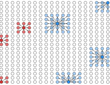
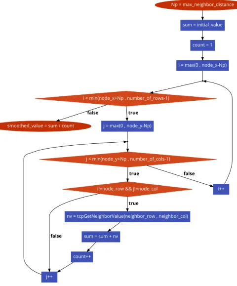
Sometimes the DSN-PC measurements contain outlier values. The reason for these can be measurement errors or local weather phenomena. If we do not handle these errors, our simple model cannot handle the big differences between adjacent grid points and will produce incorrect results. To smooth out those spikes we applied a simple averaging algorithm which is executed by each node before starting the forecast algorithm. The nodes get the initial values from their adjacent nodes and calculate the average of those and their own values. The adjacency distance can vary between 1–3 hops, thence near neighbours are always queried and distant neighbors may be queried as well. On Figure 2 the algorithm’s operation is visu- alized on a 20×20 grid. On Figure 3 the flowchart diagram of the algorithm is shown.

Figure 2: Examples of smoothing areas for different nodes with Np= 1(red) and Np= 2(blue)

2.4. The forecast algorithm

The applied distributed algorithm is based on the barotropic vorticity equation and was developed by Charney, Fjørtoft, and von Neumann (CFvN) [3]. Later, during our previous work we altered it so that it operates on a distributed sensor network.

The details of how the algorithm operates on the network nodes were covered previously [25]. Like in the previous case [28] we ran calculations on data from the period between 2019.03.21. and 2019.03.27. For each day the measurements taken at 00:00 UTC were chosen as initial values. The Mean Absolute Error (MAE) was

(6)

calculated for each forecast by

MAE= 1

18·18

∑︁18

𝑖=1

∑︁18

𝑗=1

⃒⃒𝑧500,𝑖,𝑗−𝑧_{500,𝑖,𝑗}^′ ⃒⃒,

where𝑧_{500,𝑖,𝑗}^′ is the predicted and𝑧500,𝑖,𝑗 is the measured 500 hPa geopotential 24 hours later. Due to the special way of handling the boundary grid points [3] we did not include them in the calculation of MAE.

Np = max_neighbor_distance sum = initial_value

count = 1

i = max(0 , node_x-Np)

i < min(node_x+Np , number_of_rows-1)

j = max(0 , node_y-Np) true smoothed_value = sum / count

false

j < min(node_y+Np , number_of_cols-1)

i!=node_row && j!=node_col true

i++

false

nv = tcpGetNeighborValue(neighbor_row , neighbor_col) true

j++

false sum = sum + nv

count++

Figure 3: The smoothing algorithm as executed on one node

(7)

3. Results

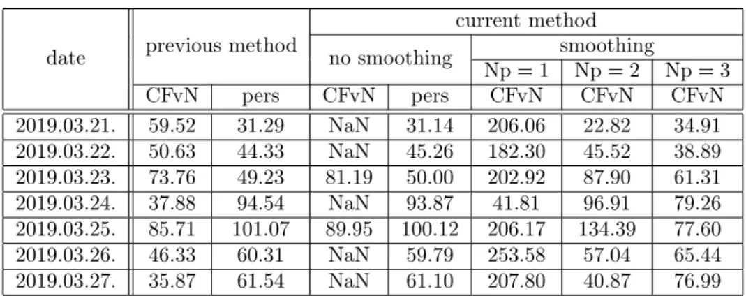
The MAE values of the forecast calculations are summarized in Table 2 where the previous (simultaneous interpolation) results [28] are also included for comparison.

The CFvN algorithm remained numerically unstable in cases where the initial data were unsmoothed and stable when smoothing was applied. The adjacency distance (Np= 1,2,3) value used during the smoothing phase had a significant impact on the goodness of the forecast. As a general rule, a minimum of Np= 2 seems to be necessary to achieve satisfactory results. On Figure 4 the initial, the analysis and the forecast height fields are shown for 2019.03.21. 00:00 UTC.

5450 5500 5550

5550 5600

5600

5600 5650

5650

5650 5650

5700

5700 5750

5750

(a) Initial height field, no smoothing

5500 5550 5600

5600 5650

5650

5650 5700

5700 5750

(b) Initial height field, smoothing with Np=2

5500 5550 5600

5600 5650

5650

5650 5700

5700

5750

5750 5800

(c) Forecast height field

5450 5500

5550

5550 5600

5600 5650

5650

5650 5700

5700 5700

5700 5750

5750

(d) Height field measured 24 hours later Figure 4: Initial height fields and the result of the CFvN forecast

performed on 2019.03.21. 00:00 UTC data

(8)

date previous method current method

no smoothing smoothing

Np= 1 Np= 2 Np= 3

CFvN pers CFvN pers CFvN CFvN CFvN

2019.03.21. 59.52 31.29 NaN 31.14 206.06 22.82 34.91 2019.03.22. 50.63 44.33 NaN 45.26 182.30 45.52 38.89 2019.03.23. 73.76 49.23 81.19 50.00 202.92 87.90 61.31 2019.03.24. 37.88 94.54 NaN 93.87 41.81 96.91 79.26 2019.03.25. 85.71 101.07 89.95 100.12 206.17 134.39 77.60 2019.03.26. 46.33 60.31 NaN 59.79 253.58 57.04 65.44 2019.03.27. 35.87 61.54 NaN 61.10 207.80 40.87 76.99

Table 2: Mean Absolute Error (m) values of the forecast calculations performed by the CFvN algorithm and the persistence method

Regarding performance, the smoothing algorithm’s execution time strongly de- pends on the network conditions, but shouldn’t take more than a few seconds.

This, in our current hardware environment, is negligible compared to the forecast algorithm’s typical execution time which is a few minutes.

4. Conclusion

We succeeded in integrating DSN-PC measurements and GFS datasets into a com- mon dataset used as initial conditions for the CFvN weather forecast algorithm.

It is a step forward from the simultaneous interpolation because of the direct integration of our data. As can be seen from the results, handling the outliers in the 2D grid is necessary while we use the CFvN algorithm. For that purpose, we successfully implemented a simple data smoothing algorithm on the virtual network nodes that can compute it by communicating with each other. This way we could achieve numerical stability in every investigated case. As a next step this smoothing method can be refined, especially on the boundaries. More complex smoothing methods can also be tested on the input data, although their conversion into distributed form can be challenging. However, the best way to improve our system would be the application of more advanced forecast models that can handle small-scale phenomena. Currently our system is not eligible to compete with more advanced and complex weather prediction models. Instead, our long-term goal is to make highly distributed weather prediction calculations possible.

Acknowledgements. We wish to thank Ficsor Endre, Perlaki Csaba, Szabó Sán- dor, Vas Ferenc and the Baptist Church of Kecskemét for providing place for our DSN-PC weather stations and thus supporting our research. We also thank SciTech Műszer Kft. for providing the possibility to use their facilities and for supporting

(9)

our work financially; and Gábor Nagy for his contribution in designing, manufac- turing and testing our weather stations’ electronic circuits.

References

[1] E. Andersson,J. N. Thépaut:Assimilation of operational data, in: Data Assimilation:

Making Sense of Observations, 2010,isbn: 9783540747024, doi:10.1007/978-3-540-74703-1_11.

[2] V. Baramidze,M. J. Lai, C. K. Shum: Spherical Splines for Data Interpolation and Fitting, SIAM Journal on Scientific Computing 28.1 (Jan. 2006), pp. 241–259, issn: 1064- 8275,

doi:10.1137/040620722,

url:http://epubs.siam.org/doi/10.1137/040620722.

[3] J. G. Charney,R. Fjørtoft,J. V. Neumann:Numerical Integration of the Barotropic Vorticity Equation, Tellus 2.4 (1950), pp. 237–254,issn: 0040-2826,

doi:10.3402/tellusa.v2i4.8607,

url:https://www.tandfonline.com/doi/full/10.3402/tellusa.v2i4.8607.

[4] W. Freeden,W. Törnig:On spherical spline interpolation and approximation, Mathe- matical Methods in the Applied Sciences 3.1 (1981), pp. 551–575,issn: 01704214,

doi:10.1002/mma.1670030139,

url:http://doi.wiley.com/10.1002/mma.1670030139.

[5] W. Freeden,M. Z. Nashed,M. Schreiner:Spherical Harmonics Interpolatory Sampling, in: 2018, pp. 267–300,

doi:10.1007/978-3-319-71458-5_11,

url:http://link.springer.com/10.1007/978-3-319-71458-5%7B%5C_%7D11.

[6] W. Freeden,M. Schreiner:Special Functions in Mathematical Geosciences: An Attempt at a Categorization, in: Handbook of Geomathematics, Berlin, Heidelberg: Springer Berlin Heidelberg, 2015, pp. 2455–2482,isbn: 9783642545511,

doi:10.1007/978-3-642-54551-1_31,

url:http://link.springer.com/10.1007/978-3-642-54551-1%7B%5C_%7D31.

[7] W. Freeden,W. Törnig:Spline methods in geodetic approximation problems, Mathemat- ical Methods in the Applied Sciences 4.1 (1982), pp. 382–396,issn: 01704214,

doi:10.1002/mma.1670040124,

url:http://doi.wiley.com/10.1002/mma.1670040124.

[8] Global Forecast System (GFS) | National Centers for Environmental Information (NCEI) formerly known as National Climatic Data Center (NCDC),

url:https://www.ncdc.noaa.gov/data- access/model- data/model- datasets/global- forcast-system-gfs(visited on 05/20/2020).

[9] A. D. Hartkamp,K. de Beurs,A. Stein,J. White:Interpolation Techniques for Climate Variables, Geographic Information Systems Series 99-01. International Maize and Wheat Improvement Center (CIMMYT), Mexico 1999. ISSN: 1405-7484 (1999).

[10] M. F. Hutchinson:Interpolating mean rainfall using thin plate smoothing splines, Inter- national Journal of Geographical Information Systems (1995),issn: 02693798,

doi:10.1080/02693799508902045.

[11] M. F. Hutchinson:Interpolation of Rainfall Data with Thin Plate Smoothing Splines -Part II: Analysis of Topographic Dependence, Journal of Geographic Information and Decision Analysis 2.2 (1998), pp. 152–167.

[12] M. F. Hutchinson:Interpolation of rainfall data with thin plate smoothing splines. Part I: Two dimensional smoothing of data with short range correlation, Journal of Geographic Information and Decision Analysis 2.2 (1998), pp. 139–151.

(10)

[13] C. H. Jarvis,N. Stuart:A comparison among strategies for interpolating maximum and minimum daily air temperatures. Part II: Interaction between number of guiding variables and the type of interpolation method, Journal of Applied Meteorology (2001),issn: 08948763, doi:10.1175/1520-0450(2001)040<1075:ACASFI>2.0.CO;2.

[14] B. I. Justusson:Median filtering: statistical properties.Two-dimensional digital signal pro- cessing II. (1981),

doi:10.1007/bfb0057597.

[15] M. Kiani:Template-based smoothing functions for data smoothing in Geodesy, Geodesy and Geodynamics (Mar. 2020),issn: 16749847,

doi:10.1016/j.geog.2020.03.003,

url:https://linkinghub.elsevier.com/retrieve/pii/S1674984720300197.

[16] W. Lahoz,B. Khattatov, R. Ménard: Data assimilation and information, in: Data Assimilation: Making Sense of Observations, 2010,isbn: 9783540747024,

doi:10.1007/978-3-540-74703-1_1.

[17] P. Lynch,X. Y. Huang:Initialization, in: Data Assimilation: Making Sense of Observa- tions, 2010,isbn: 9783540747024,

doi:10.1007/978-3-540-74703-1_9.

[18] M. New, M. Hulme, P. Jones: Representing Twentieth-Century Space–Time Climate Variability. Part I: Development of a 1961–90 Mean Monthly Terrestrial Climatology, Jour- nal of Climate 12.3 (Mar. 1999), pp. 829–856,issn: 0894-8755,

doi:10.1175/1520-0442(1999)012<0829:RTCSTC>2.0.CO;2,

url:http://journals.ametsoc.org/doi/abs/10.1175/1520-0442%7B%5C%%7D281999%7B%

5C%%7D29012%7B%5C%%7D3C0829%7B%5C%%7D3ARTCSTC%7B%5C%%7D3E2.0.CO%7B%5C%%7D3B2.

[19] M. New,D. Lister,M. Hulme,I. Makin:A high-resolution data set of surface climate over global land areas, Climate Research 21 (2002), pp. 1–25,issn: 0936-577X,

doi:10.3354/cr021001,

url:http://www.int-res.com/abstracts/cr/v21/n1/p1-25/.

[20] L. L. S.,G. Wahba:Spline Models for Observational Data.Mathematics of Computation 57.195 (July 1991), p. 444,issn: 00255718,

doi:10.2307/2938687,

url:https://www.jstor.org/stable/2938687?origin=crossref.

[21] A. Savitzky, M. J. Golay:Smoothing and Differentiation of Data by Simplified Least Squares Procedures, Analytical Chemistry (1964),issn: 15206882,

doi:10.1021/ac60214a047.

[22] Z. Shang,G. Cheng:Computational Limits of A Distributed Algorithm for Smoothing Spline, Journal of Machine Learning Research 18.108 (2017), pp. 1–37,

url:http://jmlr.org/papers/v18/16-289.html.

[23] R. Sibson:A Brief Description of Natural Neighbour Interpolation, in: Interpreting multi- variate data, 1981, pp. 21–36,isbn: 0471280399.

[24] W. Van Assche:W. Freeden, T. Gervens, and M. Schreiner, Constructive Approximation on the Sphere, with Application to Geomathematics, Journal of Approximation Theory 112.2 (Oct. 2001), pp. 324–325,issn: 00219045,

doi:10.1006/jath.2001.3607,

url:https://linkinghub.elsevier.com/retrieve/pii/S002190450193607X.

[25] Á. Vas,Á. Fazekas,G. Nagy,L. Tóth:Distributed Sensor Network for meteorological observations and numerical weather Prediction Calculations, Carpathian Journal of Electronic and Computer Engineering 6.1 (2013), pp. 56–63.

[26] Á. Vas,G. Nagy,L. Tóth:Networkable Sensor Station for DSN-PC System, Carpathian Journal of Electronic and Computer Engineering 8.2 (2015), pp. 37–40,

url:http://cjece.ubm.ro/vol/8-2015/n2/1512.22-8208.pdf.

(11)

[27] Á. Vas,L. Tóth:Evaluation of a simulated distributed sensor- and computational network for numerical prediction calculations, in: Communications in Computer and Information Science, ed. byV. M. Vishnevskiy,D. V. Kozyrev, vol. 919, Cham: Springer International Publishing, 2018, pp. 9–20,isbn: 9783319994468,

doi:10.1007/978-3-319-99447-5_2.

[28] Á. Vas,L. Tóth:Investigation of a Hybrid Sensor- and Computational Network for Nu- merical Weather Prediction Calculations, in: Communications in Computer and Information Science, ed. byV. M. Vishnevskiy,D. V. Kozyrev, vol. 1141, Cham: Springer Interna- tional Publishing, 2019, pp. 510–523,isbn: 9783030366247,

doi:10.1007/978-3-030-36625-4_41.

[29] G. Wahba:Spline Interpolation and Smoothing on the Sphere, SIAM Journal on Scientific and Statistical Computing 2.1 (Mar. 1981), pp. 5–16,issn: 0196-5204,

doi:10.1137/0902002,

url:http://epubs.siam.org/doi/10.1137/0902002.

[30] J. M. Wallace,P. V. Hobbs:Atmospheric Thermodynamics, in: Atmospheric Science, 2006, pp. 63–111,

doi:10.1016/b978-0-12-732951-2.50008-9.

[31] C. H. Woodford:An algorithm for data smoothing using spline functions, BIT 10.4 (Dec.

1970), pp. 501–510,issn: 00063835, doi:10.1007/BF01935569.

Improving the simultaneous application of the DSN-PC and NOAA GFS datasets