First derivatives of fuzzy surfaces

(1)

First derivatives of fuzzy surfaces

Jan Caha

^a

, Jiří Dvorský

^b

aDepartment of Regional Development and Public Administration, Mendel University in Brno, Zemědělská 1, 613 00, Brno, Czech Republic

jan.caha@mendelu.cz

bDepartment of Computer Science,VŠB - Technical University of Ostrava, 17. listopadu 15, 708 33 Ostrava-Poruba, Czech Republic

jiri.dvorsky@vsb.cz

Submitted October 10, 2016 — Accepted July 25, 2017

Abstract

The presented research shows how the first derivatives (slope and aspect) can be calculated from a fuzzy surface by the means of fuzzy arithmetic within the geographic information system. The proposed method works with fuzzy numbers of arbitrary shape which helps with more precise specification of input values as well as more exact calculation of results. Three most important methods of partial derivatives calculation based on finite elements approximation of a surface are presented and discussed. The presented approach provides an alternative for uncertainty propagation that is commonly performed by the utilization of statistics and the Monte Carlo method in geographic applications. The example calculation shows the differences between the obtained results calculated with the utilization of fuzzy arithmetic and the Monte Carlo method.

Keywords: fuzzy surface, fuzzy arithmetic, surface derivatives, uncertainty propagation

MSC:03B52, 26E50, 90C70

1. Introduction

The process of modelling surface from a finite set of samples is a common problem in geosciences. Surfaces are often treated as certain and error-free models [41]

even though there is a wide set of reasons why they are not. Perhaps the biggest

http://ami.uni-eszterhazy.hu

19

(2)

issue arises from incomplete knowledge about the surface under study [32]. A user cannot be sure that the sample of surface values contains values that are representative enough to construct a precise surface. There is also the issue of measurement precision of the individual sample point, some authors point out that every measurement is fuzzy, at least to some extent, because there are no absolutely precise measurements [26, 37]. Another uncertainty can be introduced to the surface by the selection of interpolation technique [32]. Not only there is a range of methods that can be used for interpolation (IDW, spline interpolators, kriging etc.) but some of these methods have parameters (e.q. tension of spline, parameters of variogram in kriging) containing epistemic uncertainty. The values of these parameters are selected by the user and their selection is partially arbitrary [27]. In fact, these parameters are better described as a set of possible values than a single value which may not be correct. Authors [25] argue that much, if not the most, of uncertainty of surfaces in geosciences is interval, fuzzy or possibilistic in its nature. Fisher [13] mentions that the fuzzy set theory should be used if the definition of a class or an individual object is vague. The individual object in the case of a surface, represented commonly in geographic information system (GIS) by a grid, is a cell and its value is definitely vague because it can be based on uncertain data, influenced by epistemic uncertainty in the interpolation method [27] and even the grid model itself is a simplification and idealization of a real surface, which introduces yet another source of uncertainty [11].

Based on these facts a model of surface that would account for its inherent uncertainty is needed [26]. Such model was firstly proposed in [8] and [4]. A fuzzy surface as described in [8] is a result of interpolation with imprecise data, while the model in [4] was based on precise data but imprecise variogram in kriging interpolation. These two studies were the first to introduce fuzzy numbers into spatial modelling and spatial prediction but the applications of fuzzy approaches for predictions and modelling were used in mathematics before [36]. Later, more techniques and approaches for the construction of fuzzy surfaces emerged, including bayesian fuzzy kriging [3], kriging with imprecise variograms was further improved [27], the inverse-distance weighting method [37], and spline interpolators [2, 26, 32].

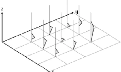
The definition of a fuzzy surface is only slightly different from an ordinary surface. A fuzzy surface is described by a set of points with knownx, y coordinates and a fuzzy numberZ˜that represents the possible values ofzat this location. The fuzzy number that describes such set of possible values represents the vague, imprecise or ill-know value. However, this uncertainty of the value does not originate in variability [25]. Similar deduction was done in [30], who mentions that statistical models often require more information about uncertainty than a user actually has. In such situations it might be reasonable and useful to formalize uncertainty in an alternative way which could be amongst others by the usage of the fuzzy set theory. Since methods for the creation of a fuzzy surface are either based on interpolation with imprecise input data, imprecise parameters of the interpolation and rarely on other methods, the outcome naturally contains this uncertainty. In- stead of storing only one value of elevation at any point of the surface, the fuzzy

(3)

surface stores a range of possible values (Fig. 1) that the surface can have at the given point. Fuzzy surfaces are an alternative to probabilistic surfaces that are commonly used in geography to estimate the influence of uncertainty on surface analyses [20, 31, 41]. While both these approaches have a lot in common there are also fundamental differences regarding the way how the resulting uncertainty is calculated and also about semantics of the results [30].

x z y

Figure 1: 3D visualization of a small fuzzy surface

The statistical approach to surface uncertainty tries to conceptualize uncertainty that occurs within the whole area of the surface through the specification of its spatial autocorrelation parameters [31]. The most commonly used method for statistical processing of uncertainty within GIS field is the Monte Carlo method [20]. Fuzzy surfaces are focused mainly on modelling uncertainty of a single cell in a grid [1, 25] while not accounting for the spatial autocorrelation explicitly. However, when the spatial autocorrelation of uncertainty is considered, it requires the user to describe it very precisely, by the specification of parameters of the autocorrelation function. This information is very rarely available to the user [30] which leads to providing of expert estimates instead of exact values [31].

As noted in [14], fuzzy mathematics has been rarely employed to actually anal- yse fuzzy surfaces, even though fuzzy surface exist ín geosciences for a long time.

However, some examples of calculations of fuzzy slopes [6, 16, 37] and the visibility analysis on fuzzy surfaces [1] exist. All of them are, however, rather a cases of specific examples that describes only one method with specific type of fuzzy surface. In this article we summarize several methods for the calculation of slope and aspect from the fuzzy surfaces that are working with the arbitrary type of fuzzy numbers. The presented methods should provide an approach for the fuzzy slope and the fuzzy aspect calculation as general as possible. Further the presented method serves as an example of a spatial analysis on a fuzzy surface and the article explains all the necessary steps needed to devise fuzzy equivalent of any subsequent analysis.

2. Fuzzy numbers and fuzzy arithmetic

A fuzzy number is a special case of a fuzzy set [40], that represents a imprecise or uncertain value. Like a fuzzy set a fuzzy numberF˜ is also defined by a membership

(4)

functionµF˜(x)that assigns the value from the interval [0,1] to every xfrom the universeX. The value ofµF˜(x)is denoted as membership value and describes how much likely it is that the given valuexbelongs to the fuzzy numberF˜. Authors [24]

explain the semantics of a fuzzy number using the concept of interval of confidence (not to be confused with the confidence interval from statistics) and the level of presumption. The level of presumption is another designation for membership value. The interval of confidence describes the range that the value can take, while the level of presumption determines how likely this interval of confidence is. As the level of presumption increases the interval of confidence never increases [24]. This association corresponds to the mechanism of human thinking about uncertain variables. The less likely values (lower presumption levels) can be found in wider intervals while the values that are more likely (higher presumption levels) are situated in narrower intervals.

There are three main conditions that a fuzzy set has to fulfil in order to be a fuzzy number [19]. The universe on which the set is defined should be real numbers – R. The height of the fuzzy set have to be equal to 1[40] so that there is at least one value with a full membership to the set. The fuzzy set has to be convex. The convex fuzzy set fulfils:

µF˜(λx1+ (1−λ)x2)≥min(µF˜(x1), µF˜(x2)) (2.1) for eachx1 andx2from Randλfrom the interval[0,1][40].

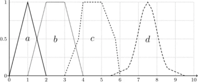
There are several types of fuzzy numbers, however the piecewise linear fuzzy numbers are of special importance here because they are simple for implementation and calculations [7, 19]. Visualization of different types of fuzzy numbers is shown in Fig. 2.

0 1 2 3 4 5 6 7 8 9 10

0 0.5 1

a b c d

Figure 2: Visualization of fuzzy numbers: a)triangular,b)trape- zoidal,c)piecewise linear,d)piecewise linear approximating gaus-

sian

There are several important notions describing fuzzy numbers:

• kernel is a set of allxwhereµF˜(x) = 1

• support is a set of allxwhereµF˜(x)>0

• α−cut is a set of all xwhere µF˜(x)≥αfor all α∈[0,1], and is denoted as F˜α

(5)

The important property is that allα-cuts (including kernel and support) are crisp sets [9, 40]. Such α-cut can be written as Fα = [Fα, Fα], where Fα is a closed interval andFα, Fα are lower and upper endpoints of this interval. This is useful for further processing of fuzzy sets. The value ofαis the level of presumption and theα-cut itself is the interval of confidence in the description provided in [24].

The decomposition theorem states that every fuzzy set can be described by a sequence of α-cuts [19]. The theorem further states that for every x ∈ R that belongs to the fuzzy setF˜ applies:

µF˜(x) = sup{α∈ h0,1i |x∈Fα}. (2.2) This theorem helps with representing the fuzzy set by a finite number ofα-cuts. It also allows the transformation from the description by membership function into the description byα-cuts and vice versa.

For practical implementations it may be necessary to describe fuzzy sets by a list of itsα-cuts then the number of such cuts has to be specified. After choosing a suitablemas the number of intervals to divide the interval[0,1]into, m+ 1values ofα-cuts is given by following equation [19]:

µj= j

m, j= 0,1, . . . , m (2.3)

Such decomposition of a fuzzy set is very useful for practical applications, especially for the calculation with fuzzy numbers.

Classic crisp numbers can be seen as a special case of fuzzy numbers, where eachα-cut is a degenerative interval ([x, x], wherex=x) [19]. This fact allows the combination of crisp values with fuzzy numbers in calculations.

2.1. Fuzzy arithmetic

Fuzzy arithmetic is an extension of a classic arithmetic on fuzzy numbers [24]. It allows complex mathematical operations with vague values. For functional combination fuzzy numbers X,˜ Y˜ the membership function of resulting fuzzy numberZ˜ is defined by the extension principle [40]:

µZ˜(z) = sup

z=F(x,y)

min(µX˜(x), µY˜(y)). (2.4) In this equation the F(x, y) is the functional combination of values xand y that belongs to fuzzy setsX˜ andY˜ respectively. Eq. (2.4) is the most general form of extension principle which can be either simplified for functions of only one fuzzy number or extended to functions of more than two fuzzy numbers [19, 24]. The extension principle provides complete theoretical foundation for the calculation of all possible operations with fuzzy numbers. However, it is not particularly suitable for the practical implementation due to its high computational demand [19].

Three alternatives to this approach exist: the concept of L-R fuzzy numbers [9], decomposed fuzzy numbers [19] and the usage of interval arithmetic for calculation ofα-cuts [19, 24, 29]. This last approach is identified as the most suitable for the practical use in [19].

(6)

2.2. Use of interval arithmetic for calculations with fuzzy numbers

The practical implementation of fuzzy arithmetic that uses interval arithmetic is based on the usage of the decomposition theorem (Eq. (2.2)). Fuzzy numbers decomposed on theirα-cuts can be combined as ordered sets of intervals according to interval arithmetic defined in [29]. The implementation can be described as a following series of steps. Fuzzy numbers X˜ and Y˜ are divided intom+ 1α-cuts (Eq. (2.3)). Then for each of thoseµj:

[Zα, Zα] = [Xα, Xα][Yα, Yα] = [min(G),max(G)] (2.5) G={XαYα, XαYα, XαYα, XαYα}. (2.6) If the operationis division, we assume that0∈/[Yα, Yα], otherwise the operation is not valid.

2.3. Functions of fuzzy numbers

The issue of propagation of fuzzy numbers through functions is much more complex than the basic fuzzy arithmetic. Still some approaches from interval arithmetic are of use and can simplify the process significantly [19]. For functions that are monotonous with respect to all their variables the problem is simple, there is only a need to the propagate combinations of endpoints ofα-cuts [29]:

f( ˜Yα) = [min(f(Xα), f(Xα)),max(f(Xα), f(Xα))] (2.7) Other functions like the integer exponentiation of a fuzzy number can be ex- plained by a set of rules [24, 29]. If the exponentnis an odd number, then:

X˜_αⁿ= ˜Zα=





 [Xα

n, Xαn]ifXα<0 [Xαn, Xα

n]ifXα>0 [min(Xαn, Xα

n),max(Xαn, Xα

n)]otherwise.

(2.8)

if the exponent is an even number:

X˜_αⁿ= ˜Zα=





 [Xα

n, Xαn]ifXα<0 [Xαn, Xα

n]ifXα>0 [0,max(Xαn

, Xα

n)]otherwise.

(2.9)

In other cases it is usually necessary to use directly the extension principle (Eq. (2.4)) or some technique that simplifies this use – i.e. the transformation method [19]. The extensive description of fuzzy arithmetic and related topics can be found in [19, 24, 29].

(7)

3. Comparison of fuzzy arithmetic and monte carlo

Utilization of the Monte Carlo method for the uncertainty propagation is rather common in surface analyses [12, 20, 21, 31], on the other hand fuzzy arithmetic is used rather rarely [14]. The main reason is because the Monte Carlo procedure is very simple to implement [19], as described in [31]. The method can be described by four main steps. The first step is to develop a model of surface and a model of uncertainty. The model of uncertainty is usually based on experts’ knowledge and reasonable assumptions about the spatial autocorrelation of uncertainty [31].

The next step is to draw enough random realizations of uncertainty and add it to the surface to produce the uncertain surface. For each realization the calculation of analysis (e.g. slope, aspect, visibility calculation) is performed. The last step is to statistically evaluate the results, usually by calculating mean and standard deviation of the results. The process itself does not require any changes to the calculation of analysis, only its repetition for several times. The method is only demanding on computational power and time, because the number of iterations is generally in hundreds or even thousands.

The utilization of fuzzy arithmetic requires the adjustment to the analysis algorithms, because it has to be done according to the principles of fuzzy arithmetic.

So far fuzzy arithmetic is not implemented in any software that would allow calculations of anything else but very simple examples. This is one of the reasons why the use of fuzzy arithmetic is at present limited to the scientific studies [19]. In case of the surface analysis, uncertainty of the surface is directly included in the fuzzy surface, so there is no need to generate random realizations of the surface and the result is calculated in one pass, without the need to iteratively calculate the outcomes.

Fuzzy arithmetic and the Monte Carlo method serve the same purpose – the uncertainty propagation. However, semantics and procedures vary significantly.

The biggest difference is in both semantics of the result and its range. Since Monte Carlo is based on probability, it focuses on obtaining the probable outcomes and it cannot guarantee that the results will include all possible outcomes. Fuzzy arithmetic is focused on obtaining all the possible outcomes, so it guarantees that even the extreme combinations of input values will be included in the result. This is the main difference that arises from semantic differences between the Monte Carlo method (probabilistic model of uncertainty) and fuzzy arithmetic (model of uncertainty based on imprecision). The more developed analysis of semantics differences amongst the uncertainty theories is provided in [30].

The Monte Carlo method can be adjusted to produce results that are actually close to the results of fuzzy arithmetic, by use of optimization methods like for example the latin hypercube sampling [28]. But the usage of these optimization techniques in geosciences is not common. Indeed, fuzzy arithmetic provides results that yield larger uncertainties, however, if there is very little knowledge about uncertainty, it is the semantically correct approach [30].

(8)

4. Derivatives of surfaces

Derivatives are useful characteristics as they are providing a mathematical description of the surface appearance. The GIS tools for their calculation are based on the approximation of a real surface by a finite number of elements [39]. In the case of a grid structure these elements are cells [37]. This means that the derivative at a specific cell is calculated based on the values of neighbouring cells. There are two first derivatives of the surface: slope and aspect, several second derivatives that describe various types of curvature [39], a complete list of primary and secondary surface parameters and their significance is provided in [38]. All of those are commonly used in geographical and environmental analyses, for example in the fields like hydrology, geomorphology, geology, oceanography, ecology and others [34].

According to [39], two conditions have to be met to allow the calculation of the derivatives of the surface. The cells of the grid have to be aligned to the geographical axes and the distance between the centres of the cell should be the same for the whole grid. If both these conditions are met, the calculation is rather straightforward. Otherwise it is necessary to resample the grid according to those conditions. Other solution would be the modification of the equations which is performed rather rarely due to the complexity of this process [39].

z

1

z

2

z

3

z

4

z

5

z

6

z

7

z

8

z

9

Figure 3: Node numbering convention in the neighbourhood of a central cellz9 (edited from: [39])

4.1. Methods of derivatives calculation

The basis of the derivatives determination is to calculate partial derivatives of the surface in two directions: North-South (denoted as^∂z_∂y with respect to the alignment with this axis) and East-West (denoted as ^∂z_∂x). There are several methods for calculation of those gradients, their comparison was performed in [23], [42] and also in [34]. The conclusion was that the 4-Cell method [15] provides the most precise results, closely followed by the Horn’s method [22]. The third best algorithm was a modified version of Horn’s method and as the forth the method of Sharpnack and Akin [33] was evaluated [23], these conclusions are approximately in agreement with the conclusions made in [34]. Study [42] was focused mainly on other elements of calculation. The algorithms were tested with respect to data quality and the resolution of the grid but findings from all these papers [23, 34, 42] suggest that

(9)

4-Cell, Horn’s, Sharpnack’s and Akin’s methods are all good estimators of the first derivatives of the surface. Based on these results, these three algorithms for gradient calculation are considered in the article, they happen to be the most commonly implemented in GIS.

In all upcoming formulas the cells are labelled according to Fig. 3. The variable d denotes the size of the grid cell. The arrangement and numbering of the cells vary through the literature and the formulas for calculation of the derivations vary accordingly [39].

The 4-Cell method calculates the values of gradients only from the cells that have direct neighbourhood with the central cell. The method was firstly described in [15]. The equations for this calculation are:

∂z

∂x = z2−z6

2d , (4.1a)

∂z

∂y = z8−z4

2d . (4.1b)

Horn’s method considers even the cells in the neighbourhood that have only one point common with the central cell. Cells that have common edge have been assigned higher weight in the calculation. The method was presented in [22] and the equations are:

∂z

∂x = (z1+ 2z2+z3)−(z7+ 2z6+z5)

8d , (4.2a)

∂z

∂y = (z7+ 2z8+z1)−(z5+ 2z4+z3)

8d . (4.2b)

Sharpnack and Akin’s Method is very similar to the Horn’s method with the change that all cells have the same weight. This method was proposed in [33] and the equations have the following form:

∂z

∂x =(z1+z2+z3)−(z7+z6+z5)

6d , (4.3a)

∂z

∂y =(z7+z8+z1)−(z5+z4+z3)

6d . (4.3b)

4.2. Calculation of slope and aspect

The three methods that were mentioned in the previous section provide three ways for the gradient calculation. These gradients are further used to calculate the slope S and the aspectA. For the slope calculation as a proportional rise the following equation is used:

S = s∂z

∂x 2

+ ∂z

∂y 2

. (4.4)

(10)

If the result should be in percent, a slightly different variation of the equation is needed:

S= 100 s∂z

∂x ²

+ ∂z

∂y ²

. (4.5)

If the result should be provided in degrees, a slight modification is necessary. This slope is labelled as geographical:

Sg (^◦) =180 π arctan



s

∂z

∂x 2

+ ∂z

∂y 2

. (4.6)

The calculation of aspect is a bit more complicated and requires the use of arctan2function:

A= arctan2(−∂z

∂y,−∂z

∂x). (4.7)

The mathematical aspectAis different from the geographical aspectAg,Ahas a range of [−π, π] radians, the value of 0 for the East and the values increase in a counter-clockwise direction. Ag has a range of [0,2π] in radians or [0^◦,360^◦] in degrees, the value of0for the North and the values increase in a clockwise direction [39]. So there is a need to adjust the values by this formula:

Ag (^◦) =

(450^◦−¹⁸⁰π A if ¹⁸⁰_π A >90^◦

90^◦−¹⁸⁰π A otherwise. (4.8)

Based on those equations the calculation of approximation of slope and aspect can be calculated from the surface represented by the grid.

5. First derivatives of fuzzy surfaces

In any analysis calculated on a fuzzy surface uncertainty of the surface is propagated through the analysis into the result. Such result then shows uncertainty connected to the input data represented as fuzzy numbers. So far there are three examples of the calculation of a fuzzy slope in the literature provided in [16], [37] and [6].

Unfortunately, in first two cases a fuzzy slope is not the main focus of the research so it is not discussed in detail. [16] use a fuzzy slope to identify the areas having a slope potentially higher than25 %, but the calculation serves as one of the several examples in the article, so it is discussed very briefly. [37] provided methods for the calculation of partial derivatives using the finite elements method, but the presented method is focused on a fuzzy surface constructed using purely triangular fuzzy numbers. The equations are adjusted to work on such surface, but it does not handle the calculation of a fuzzy slope in general, because triangular fuzzy numbers are only one type of a theoretically infinite set of fuzzy number types. These case

(11)

specific adjustments of equations are common for presenting methods that utilize fuzzy arithmetic [19]. [6] described the calculation of only fuzzy slope using Horn’s algortihm. There has been no attempt (of which the authors are aware) to calculate the aspect of a fuzzy surface.

The basis for the determination of both slope and aspect is the calculation of gradients ^∂z_∂x and ^∂z_∂y. Considering that all inputs are uncertain and represented by fuzzy numbers, the results will also contain uncertainty and they will also be represented by fuzzy numbers. The calculation of gradients themselves is based on basic arithmetic operators that have fuzzy equivalents according to Eqs. (2.2, 2.3) and ((2.5, 2.6). This applies for all three methods of the gradient calculation (Eqs.

(4.2, 4.1, 4.3)).

5.1. Slope

Calculating slope of a fuzzy surface according to Eqs. (4.5, 4.6) does not need any special approaches. Square of a fuzzy number can be calculated according to Eq.

(2.8) and square root is a monotonous function and can be calculated according to Eqs. (2.2) and (2.7). If the slope is to be provided in degrees then the Eq. (4.6) is used. As mentioned previously, there is no problem with using crisp numbers with fuzzy numbers while calculating. Thus obtaining the value of the slope as a fuzzy number is a relatively simple matter.

5.2. Aspect

The aspect calculation is more complicated then the slope calculation. The Eq.

(4.7) contains the function arctan2 [18] that has to be calculated for two fuzzy arguments. This in not a trivial operation and the function has to be modified to allow the calculation. The common definition ofarctan2is:

arctan2(y, x) =











arctan^y_x ifx >0

arctan^y_x+π ify≥0andx <0 arctan^y_x−π ify <0andx <0 +^π₂ ify >0andx= 0

−^π2 ify <0andx= 0 undefined ify= 0andx= 0

(5.1)

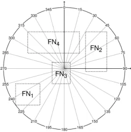
From the viewpoint of the calculation with fuzzy numbers there are two main problems. The function is not defined fory= 0andx= 0and it is discontinuous for x > 0 and y = 0 (Fig. 5). This complicates the calculation if Y˜ and X˜ contain 0. Figure 4 shows four examples of areas bounded by supports of fuzzy numbers, labelled FN1, FN2, FN3 and FN4. As visible from the examples, FN1

and FN2 delimit angle intervals with the values of approximately [215^◦,250^◦] and [30^◦,100^◦].¹ Example FN3 shows a situation in which both intervals contain 0

1The presented examples are for the sake of understanding shown in degrees with0^◦pointing

(12)

and as a result FN3 has a range of [0^◦,360^◦], which practically means that the aspect cannot be specified. The most interesting situation is FN4, the smallest value contained in the rectangle is 0^◦ and the highest value is 360^◦ but actually the values between 45^◦ and 290^◦ do not belong to the set. In such situation it is impossible to construct a valid fuzzy number with respect to Eq.(2.1).

0 15

30 45

60

75

90

105

120

135 150 180 165

195 210 225 240 255 270

285 300

315 330

345

FN₁

FN₂ FN₃

FN₄

Figure 4: Four examples of bounding boxes on orientation

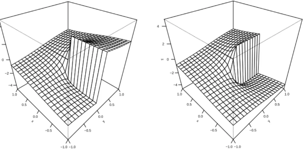
In order to allow the calculation with fuzzy numbers there is a need for a modified version of the function. As noted in [18] there exists a zero direction problem in directional statistics, the problem that is encountered whenarctan2is calculated for the fuzzy arguments is quite similar. It can be avoided but the obtained results will require a little bit more work in order to be interpreted correctly.

arctan2m(y, x) =











arctan^y_x−2π ify≤0andx >0 arctan^y_x ify <0andx >0 arctan^y_x−π ify≥0andx <0 arctan^y_x−π ify <0andx <0 +^π₂ −π ify >0andx= 0

−^π2 −π ify <0andx= 0 undefined ify= 0andx= 0

(5.2)

If the calculation of arctan2( ˜Y ,X˜)is to be performed, firstly it needs to be deter- mined if the problem with discontinuity of the function will occur. This will happen if for any αthere exist α-cuts such that0 ∈Y˜α and 0>X˜α. If this condition is true, the modified version of arctan2 needs to be used (Eq. (5.2)). The rotated

upward and clockwise rise, even though those angles should be in radians with0pointing to the left and counter-clockwise rise of values.

(13)

variant of the function has a modified range [−1.5π,0.5π] instead of the original range[−π, π] and it is discontinuous ifx= 0andy <0 (see Fig. 5). The problem with undefined value of both functions is solved by setting the result interval to a full range of values if x= 0and also y= 0. In either case both functions arctan2 and arctan2mare continuous with respect to both variables and as such they can be propagated by the use of simple approach according to Eq. (2.7).

y

−1.0

−0.5 0.0

0.5 1.0

x

−1.0

−0.5 0.0 0.5 1.0 z

−4

−2 0 2 4

y

−1.0

−0.5 0.0

0.5 1.0

x

−1.0

−0.5 0.0 0.5 1.0 z

−4

−2 0 2 4

Figure 5: Left figure – values ofarctan2(y, x). Right figure – values ofarctan2m(y, x). Values ofZ are in radians

When recalculating from the mathematical orientation onto the compass orientation (Eq.(4.8)), the value used for the comparison is the maximal value of the kernel –A1. After calculatingAgaccording to Eq. (4.8), the resulting values ofAg

then do not fit in the original range of aspect values[0^◦,360^◦], which is the result of the propagation of fuzzy numbers through the calculation. Actually, the resulting values are from the range of [−90^◦,630^◦], meaning that the negative values v have the aspect of360^◦+v and the positive values v higher than 360^◦ are equal tov−360^◦. The fuzzy orientation is more complicated for interpretation, but it is necessary to calculate them as such values to allow the correct propagation of the fuzzy numbers through the calculation. For the visualization and interpretation it is necessary to ensure that all those values will be interpreted correctly.

6. Numerical example

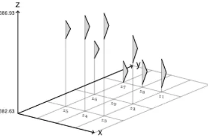
In this section an example of the calculation of aspect and slope using Horn’s method (Eq. (4.2)) will be shown. The method is chosen because it is the one that is most commonly implemented in GIS. For the sake of readability the calculation will only be done for α-cuts0 and1. Each alpha cut of the fuzzy numberF˜ will be written as (α : ˜Xα; ˜Xα). The distance between cells has a value of d = 10 meters. The input fuzzy numbers or neighbouring cells are triangular and have the

(14)

following definition:

z1= (0.0 : 382.81; 384.01)(1.0 : 383.41; 383.41) z2= (0.0 : 384.34; 385.5)(1.0 : 384.92; 384.92) z3= (0.0 : 385.83; 386.93)(1.0 : 386.38; 386.38) z4= (0.0 : 385.63; 386.63)(1.0 : 386.13; 386.13) z5= (0.0 : 385.46; 386.22)(1.0 : 385.84; 385.84) z6= (0.0 : 384.13; 384.87)(1.0 : 384.5; 384.5) z7= (0.0 : 382.63; 383.53)(1.0 : 383.08; 383.08) z8= (0.0 : 382.74; 383.78)(1.0 : 383.26; 383.26)

The surface used in this example is visualized in Fig. 6.

x y z

382.63 386.93

z5 z4

z3 z6

z9 z2 z7

z8 z1

Figure 6: Visualization of a small fuzzy surface used in the example

The first step is to calculate the values of ^∂z_∂x and ^∂z_∂y, to do that we firstly extract the necessary α-cuts from the fuzzy numbers according to Eq. (2.3) and then calculate the values according to Eq. (4.2) for eachα-cut, applying Eqs. (2.5, 2.6) for each operation. The resulting fuzzy numbers have the values of:

∂z

∂x = (0.0 :−0.027; 0.07)(1.0 : 0.021; 0.021)

∂z

∂y = (0.0 :−0.19;−0.09)(1.0 :−0.14;−0.14).

With the knowledge of gradients the calculation of slope is a simple matter (Eq.

(4.5)). Eq. (2.8) will be used to calculate the power of fuzzy numbers, the addition of fuzzy numbers is done according to Eqs. (2.5, 2.6) and square root can be calculated as a monotonous function (Eq. (2.7)).

∂z

∂x

2

= (0.0 : 0.0; 0.005)(1.0 : 0.00; 0.00)

∂z

∂y

2

= (0.0 : 0.009; 0.037)(1.0 : 0.02; 0.02)

(15)

S= (0.0 : 0.093; 0.206)(1.0 : 0.145; 0.145)

The value of slopeScan be further transformed to percent according to Eq. (4.5):

S= (0.0 : 9.3; 20.6)(1.0 : 14.5; 14.5).

To calculate the aspect the Eq. (4.7) will be used.

A= (0.0 : 73.74; 126.92)(1.0 : 98.48; 98.48)

The mathematical aspect needs to be turned into the geographical aspect according to Eq. (4.8). For the comparison the value ofA1is used and the geographical aspect is obtained.

Ag= (0.0 :−36.92; 16.26)(1.0 :−8.48;−8.48)

As can be seen this is the case when the range of the resulting fuzzy easpect is outside of the classic aspect range [0^◦,360^◦]. That means that this fuzzy aspect needs to be used interpreted as described in section 5. The resulting geographical aspect spans around north, with the modal value being slightly inclined towards west. For the further comparison with Monte Carlo method the range of the result can be described by two intervals [0,16.26],[323.08,360] (^◦) that have the same interpretation as the support of fuzzy aspect.

Through the whole presented example for all variables the kernel value of each fuzzy number is the same as it would be in case of the calculation with crisp values.

This fact shows that the propagation was done correctly because if triangular fuzzy numbers, where the kernel value corresponds to what originally was a crisp number, are used, then the kernel value of the result should be equal to the result of crisp calculation [19].

As a comparison the same calculations were performed with the use of the Monte Carlo simulation, using 100, 500, 1 000, 10 000 and 1 000 000 iterations.

Triangular probability distributions were used as they are specified by three values [10], which makes them very similar to the triangular fuzzy numbers. The results of the simulations are summarized in Tab. 1. It is obvious that as the number of simulations raises, the ranges get closer to the range identified by fuzzy arithmetic.

But it is very unlikely, even with very high number of simulations, for Monte Carlo to identify a complete range of possible outcomes.

The results that Monte Carlo failed to identify have very small probability of occurrence, but that are feasible solutions to the problem, this result is in agreement with the examples provided by [19] and [25]. These solutions can be perceived as the best/worst possible solutions and they can possibly be important for decision making. The complete range of outcomes should be [9.3,20.6](%) for the slope and[0,16.26],[323.08,360](^◦) for the aspect.

The Monte Carlo method did not reach these widths of intervals but it is visible from the Tab. 1 that as the number of simulations increases, the estimates are actually converging towards the results provided by fuzzy arithmetic. However,

(16)

Table 1: Monte Carlo experiments

Simulations Slope range (%) Aspect range (^◦) 100 [12.23,16.54] [344.24,359.83]

500 [12.08,17.16] [0.01,1.28],[339.93,359.77]

1 000 [11.43,17.33] [0.06,2.24],[341.30,359.92]

10 000 [11.21,17.84] [0.06,2.81],[339.54,359.54]

1 000 000 [10.61,18.27] [0.00,5.93],[336.03,360.00]

the number of simulations to obtain the true range is likely to be very high since the extension of the intervals is not significant even for a significant increase in the number of simulations. E.g. the change between the fourth and the fifth row of Tab. 1, even though the number of simulations is increased by a factor of 100 the obtained results change relatively insignificantly.

The calculation of slope and aspect for a whole grid instead of just one cell requires simply repeating this step for each cell of a grid. The source code for calculations of fuzzy derivatives with higher number of α-cuts and the other two methods for derivatives calculation are referenced in the Appendix 8.

7. Case study: Analysis of artificial fuzzy surface

For the purpose of practical demonstration analysis of fuzzy surface the artificial dataset is used. The dataset itself as well as code for its creation is described in Appendix 8. The case study demonstrates practical usability of fuzzy surface analyses in geographical applications.

Points from which the fuzzy surface is created are generated as Gaussian random field with gaussian correlation function with sill 200, range 400, nugget 0 and mean value equal to 150. To make the data less dependant on the specific function a random value drawn from normal distribution with 0 mean and standard deviation equal to 4 is added to each point. The dataset consists of 400 measurements randomly distributed in the area of size 4000×4000 meters. Thezvalue (elevation) is interpolated into a grid of 401×401 cells, which makes cell size equal to 10. This datasets simulates real data measured on a surface.

The dataset is interpolated using fuzzy kriging with uncertain variogram proposed originally in [4] and later further developed in [27]. The kriging parameters sill, range and nugget are specified as triangular fuzzy numbers. The specific values are summarized in Tab. 2. The process of calculation of fuzzy kriging as well as source code for fuzzy interpolation are presented in [5].

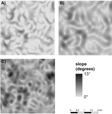
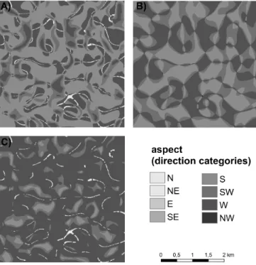
Based on the previously mentioned fuzzy surface the fuzzy slope and fuzzy aspect can be calculated using procedures shown in section 5. For further use the values of minimum, modal a maximum are the most important as they describe the limits and the most likely value. The visualizations of fuzzy slope and fuzzy

(17)

Table 2: The values of semivariogram parameters Parameter Minimal value Modal value Maximal value

sill 130 138 145

range 390 395 400

nugget 13 15 17

aspect calculated with use of Horn’s derivatives equations (Eq. (4.2)) are on Figs.

7 and 8.

Figure 7: Visualization of minimal (A), modal (B) and maximal (C) slope calculated from the fuzzy surface. The slope unit are

degrees

The presented approach is useful in analysing uncertain surfaces, where it would be illogical to present precise outcomes. For example the if the geostatistical esti- mations based on imprecise information, as presented in [35], should be analysed then using fuzzy arithmetic is the only proper way to do so.

(18)

Figure 8: Visualization of minimal (A), modal (B) and maximal (C) aspect calculated from fuzzy surface. The aspect is visualized

in directional categories

8. Conclusion

Hanss [19] noted that fuzzy arithmetic has received little attention and that the applications barely exceeded the level of elementary academic examples. The same statement regarding the analyses of fuzzy surfaces is done in [14]. The main reason for this lack of practical utilization is that there is basically no implementation of fuzzy arithmetic in even the mathematical software let alone within GIS. Excep- tions are relatively new tools for R project FuzzyNumbers [17] and also FuzzyKrig toolbox [35] for Matlab^R. The former allows calculations with fuzzy numbers while the latter is a tool for spatial interpolation with uncertain data and/or uncertain parameters. The secondary reason could be that some operations are not straightforward, like the presented calculation of aspect of a fuzzy surface. The process is more complex when compared to the commonly used Monte Carlo method. But still, such analyses are possible and necessary for further progress in the topic of analyses of fuzzy surfaces.

The presented research is in agreement with the previously performed studies that presented the processes of slope calculation [6, 16, 37], above that the procedure for calculating the aspect of a fuzzy surface is presented as well. The

(19)

presented algorithms work for fuzzy numbers of arbitrary shape and the precision of the calculation can be adjusted by selecting different amounts ofα-cuts. Three types of surface gradients that are the most commonly implemented in software were shown to be compatible with fuzzy arithmetic and can be used to calculate the first derivatives of fuzzy surfaces.

The advantage of the presented approach, when compared to another commonly used technique of the uncertainty propagation – the Monte Carlo method, is that the derivatives of a surface are calculated in one pass and all uncertainty of the fuzzy surface is included in the result. Uncertainty is naturally incorporated in the process by the use of fuzzy numbers and fuzzy arithmetic, so there is no need for iterations in the calculation. Unlike Monte Carlo, fuzzy arithmetic can guarantee inclusion of all possible outcomes (including limit cases) in the result. The Monte Carlo method, on the other hand, focuses only on the most probable results [19].

This is an important difference amongst these two methods that might be important for decision making process based on the result of calculation with uncertainty.

According to the extension principle [40], every operation can be extended to its fuzzy equivalent. That means that every analysis that can be performed on a surface in GIS can be also performed on a fuzzy surface and the result will contain and bound uncertainty of the surface. Such approach to modelling should provide an alternative to the currently used Monte Carlo method and provide GIS users another possibility how to conceptualize and propagate uncertainty through geographic analyses. The need for new approaches and methods is quite significant as the issue of uncertainty propagation within GIS is still relatively undeveloped [21].

Further research should focus on a subsequent surface analysis, which can include but are not limited to second derivatives, optimal path selection, visibility analysis, catchment delimitation and others.

Acknowledgements Authors are thankful for the reviewers’ comments that helped in improving this article.

Appendix: Code

The examples in section 6 are performed with the use of FuzzyNumbers package [17]. The source code for the example and its variants, calculated using different method of derivatives determination, can be found in https://github.com/

JanCaha/AMeI-paper. The data used in section 7 are available as well along with the results calculated by other two methods for gradient calculation.

Procedure of creating the fuzzy surface that was used as input data in the case study can be found inhttps://github.com/JanCaha/Hais2015-paperand in [5].

(20)

References

[1] A. M. Anile, P. Furno, G. Gallo, and A. Massolo. A fuzzy approach to visibility maps creation over digital terrains. Fuzzy Sets and Systems, 135(1):63–80, 2003.

[2] A. M. Anile and S. Spinella. Modeling Uncertain Sparse Data with Fuzzy B-splines.

Reliable Computing, 10(5):335–355, 2004.

[3] H. Bandemer and A. Gebhardt. Bayesian fuzzy kriging. Fuzzy Sets and Systems, 112(3):405–418, 2000.

[4] A. Bardossy, I. Bogardi, and W. E. Kelly. Kriging with imprecise (fuzzy) variograms.

I: Theory. Mathematical Geology, 22(1):63–79, 1990.

[5] J. Caha, L. Marek, and J. Dvorský. Predicting PM10 Concentrations Using Fuzzy Kriging. In E. Onieva, I. Santos, E. Osaba, H. Quintián, and E. Corchado, editors,Hybrid Artificial Intelligent Systems SE - 31, volume 9121 ofLecture Notes in Computer Science, pages 371–381. Springer International Publishing, 2015.

[6] J. Caha, P. Tuček, A. Vondráková, and L. Paclíková. Slope Analysis of Fuzzy Surfaces.

Transactions in GIS, 16(5):649–661, 2012.

[7] L. Coroianu, M. Gagolewski, and P. Grzegorzewski. Nearest piecewise linear approximation of fuzzy numbers. Fuzzy Sets and Systems, 233:26–51, 2013.

[8] P. Diamond. Fuzzy Kriging. Fuzzy Sets and Systems, 33(3):315–332, 1989.

[9] D. Dubois and H. Prade. Fuzzy sets and systems : theory and applications. Num- ber Nf. Academic Press, New York, 1980.

[10] M. Evans, N. Hastings, and B. Peacock. Triangular Distribution. In Statistical Distributions, pages 187–188. Wiley-Interscience, New York, 3rd ed. edition, 2000.

[11] P. Fisher. The pixel : A snare and a delusion. International Journal of Remote Sensing, 18(3):679–685, 1997.

[12] P. Fisher. Improved Modeling of Elevation Error with Geostatistics. GeoInfomatica, 2(3):215–233, 1998.

[13] P. F. Fisher. Models of uncertainty in spatial data. In P. Longley, M. F. Goodchild, D. J. Maguire, and D. W. Rhind, editors,Geographical Information Systems: Princi- ples, Techniques, Management, and Applications, chapter 13, pages 191–205. Wiley, New York, NY, 2nd edition, 2005.

[14] P. F. Fisher and N. J. Tate. Causes and consequences of error in digital elevation models. Progress in Physical Geography, 30(4):467–489, 2006.

[15] M. Fleming and R. M. Hoffer. Machine processing of landsat MSS data and DMA topographic data for forest cover type mapping, Laboratory for Applications of Remote Sensing. Purdue University, 1979.

[16] C. C. Fonte and W. A. Lodwick. Modelling the Fuzzy Spatial Extent of Geographical Entities. In F. Petry, V. B. Robinson, and M. A. Cobb, editors,Fuzzy modeling with spatial information for geographic problems, pages 120–142. Springer, Berlin, 2005.

[17] M. Gagolewski and J. Caha. A Guide to the FuzzyNumbers Package for R. Technical report, 2015.

[18] G. L. Gaile and J. E. Burt. Directional Statistics. Geo Abstracts, University of East Anglia, 1980.

(21)

[19] M. Hanss.Applied Fuzzy Arithmetic : An Introduction with Engineering Applications.

Springer-Verlag, Berlin ; New York, 2005.

[20] G. B. M. Heuvelink.Error Propagation in Environmental Modelling with GIS. Taylor

& Francis Ltd, London, 1998.

[21] G. B. M. Heuvelink. Analysing Uncertainty Propagation in GIS: Why is it not that Simple? In G. M. Foody and P. M. Atkinson, editors,Uncertainty in remote sensing and GIS, pages 155–165. Wiley, Chichester, 2002.

[22] B. Horn. Hill shading and the reflectance map.Proceedings of the IEEE, 69(1):14–47, 1981.

[23] K. H. Jones. A comparison of algorithms used to compute hill slope as a property of the dem. Computers & Geosciences, 24:315–323, 1998.

[24] A. Kaufmann and M. M. Gupta. Introduction to Fuzzy Arithmetic. Van Nostrand Reinhold Company, New York, 1985.

[25] W. Lodwick, A. M. Anile, and S. Spinella. Introduction. In W. Lodwick, editor,Fuzzy surfaces in GIS and geographical analysis : theory, analytical methods, algorithms, and applications, pages 1–46. CRC Press, Boca Raton, 2008.

[26] W. A. Lodwick and J. Santos. Constructing consistent fuzzy surfaces from fuzzy data. Fuzzy Sets and Systems, 135(2):259–277, 2003.

[27] K. Loquin and D. Dubois. Kriging with Ill-Known Variogram and Data. In A. Desh- pande and A. Hunter, editors,Scalable Uncertainty Management SE - 5, volume 6379 ofLecture Notes in Computer Science, pages 219–235. Springer Berlin / Heidelberg, 2010.

[28] M. McKay, R. Beckman, and W. Conover. A comparison of three methods for selecting values of input variables in the analysis of output from a computer code.

Technometrics, 21(2):239–245, 1979.

[29] R. E. Moore, R. B. Kearfott, and M. J. Cloud. Introduction to interval analysis.

Society for Industrial and Applied Mathematics, Philadelphia, PA, 2009.

[30] M. Oberguggenberger. The mathematics of uncertainty: models, methods and inter- pretations. In W. Fellin, H. Lessmann, M. Oberguggenberger, and R. Vieider, editors, Analyzing Uncertainty in Civil Engineering, page 252. Springer, Berlin, 2005.

[31] J. Oksanen and T. Sarjakoski. Error propagation analysis of DEM-based drainage basin delineation.International Journal of Remote Sensing, 26(14):3085–3102, 2005.

[32] J. Santos, W. A. Lodwick, and A. Neumaier. A New Approach to Incorporate Uncertainty in Terrain Modeling. In M. Egenhofer and D. Mark, editors,Geographic Information Science, volume 2478 ofLecture Notes in Computer Science, pages 291–

299. Springer Berlin Heidelberg, 2002.

[33] D. A. Sharpnack and G. Akin. An algorithm for computing slope and aspect from elevations. Photogrammetric Engineering, 35:247–248, 1969.

[34] A. K. Skidmore. A comparison of techniques for calculating gradient and aspect from a gridded digital elevation model. International journal of geographical information systems, 3(4):323–334, 1989.

[35] S. Soltani-Mohammadi. FuzzyKrig: a comprehensive matlab toolbox for geostatistical estimation of imprecise information. Earth Science Informatics, 2015.

(22)

[36] H. Tanaka, S. Uejima, and K. Asai. Linear Regression Analysis with Fuzzy Model.

IEEE Transactions on Systems, Man and Cybernetics, 12(6):903–907, 1982.

[37] O. Waelder. An application of the fuzzy theory in surface interpolation and surface deformation analysis. Fuzzy Sets and Systems, 158(14):1535–1545, 2007.

[38] J. P. Wilson. Digital terrain modeling. Geomorphology, 137(1):107–121, 2012.

[39] J. P. Wilson and J. C. Gallant. Terrain analysis : principles and applications. Wiley, New York, 2000.

[40] L. A. Zadeh. Fuzzy Sets. Information and Control, 8(3):338–353, 1965.

[41] J. Zhang and M. F. Goodchild. Uncertainty in geographical information. Taylor &

Francis, London, 2002.

[42] Q. M. Zhou and X. J. Liu. Analysis of errors of derived slope and aspect related to DEM data properties. Computers & Geosciences, 30(4):369–378, 2004.