materials
Article
The Effect of Crystal Defects on 3D High-Resolution Diffraction Peaks: A FFT-Based Method
Komlavi Senyo Eloh1,2,3, Alain Jacques1,2,*, Gabor Ribarik1,4and Stéphane Berbenni1,3
1 Laboratory of Excellence on Design of Alloy Metals for low-mAss Structures (DAMAS), Universitéde Lorraine, f-57073 Metz, France; komlavi-senyo.eloh@univ-lorraine.fr (K.S.E.);
ribarik@elte.hu (G.R.); stephane.berbenni@univ-lorraine.fr (S.B.)
2 Institut Jean Lamour (IJL), Universitéde Lorraine, CNRS, f-54000 Nancy, France
3 Laboratoire d’Etude des Microstructures et de Mécanique des Matériaux (LEM3), Universitéde Lorraine, CNRS, f-57073 Metz, France
4 Department of Materials Physics, Eötvös University, h-1117 Budapest, Hungary
* Correspondence: alain.jacques@univ-lorraine.fr; Tel.: +33-3-7274-2679
Received: 28 June 2018; Accepted: 31 August 2018; Published: 9 September 2018
Abstract: Forward modeling of diffraction peaks is a potential way to compare the results of theoretical mechanical simulations and experimental X-ray diffraction (XRD) data recorded during in situ experiments. As the input data are the strain or displacement field within a representative volume of the material containing dislocations, a computer-aided efficient and accurate method to generate these fields is necessary. With this aim, a current and promising numerical method is based on the use of the fast Fourier transform (FFT)-based method. However, classic FFT-based methods present some numerical artifacts due to the Gibbs phenomenon or “aliasing” and to “voxelization”
effects. Here, we propose several improvements: first, a consistent discrete Green operator to remove “aliasing” effects; and second, a method to minimize the voxelization artifacts generated by dislocation loops inclined with respect to the computational grid. Then, we show the effect of these improvements on theoretical diffraction peaks.
Keywords: dislocations; diffraction; fast Fourier transform (FFT)-based method; discrete green operator; voxelization artifacts; sub-voxel method; simulated diffraction peaks; scattered intensity
1. Introduction
X-ray diffraction (XRD) is one of the most powerful non-destructive tools to investigate materials, as their wavelength is commensurate with the distance between atoms within a crystal [1–9].
Successive improvements of both the X-ray sources (from X-ray tubes to third generation synchrotrons) and detectors (from photographic plates and gas counters to fast two-dimensional arrays) have led to a tremendous increase in the quantity of data recorded per unit time, allowing real time in situ or in operando measurements [10,11]. It is now possible to determine the 3D grain microstructure of a bulk material with a submicron resolution (using topo-tomography), to follow the evolution of the elastic strain state of the grains of a polycrystal during mechanical tests (3D-XRD, far field diffractometry), or to measure the distribution of strains within a few grains in real time (2D diffractometry) [12,13].
Such experiments result in terabytes of data recorded within a few days, which need to be analyzed efficiently. In fact, only a low fraction of those data is actually treated because scientists lack both time and numerical tools (software) for further analysis [14].
The classical techniques used to analyze the 1D or 2D diffraction patterns recorded during tests performed on polycrystalline specimens such as the Rietveld method, the square sines method to measure internal stresses, or CMWP (convolutional multiple whole profile) fitting for
Materials2018,11, 1669; doi:10.3390/ma11091669 www.mdpi.com/journal/materials
Materials2018,11, 1669 2 of 14
dislocations content often rely on simplified and mathematically tractable models of a microstructure.
Calculations which may involve a simplifying hypothesis lead to a general formula which can be used to fit one or several parameters of the microstructure (dislocation densities and type, internal stress tensor etc.) to the diffraction pattern (peak profiles, variation of the 2θBangle with orientation etc.).
During the last 10 years, several authors proposed the opposite approach: forward modeling [15–22].
This requires the design of a microstructure and the simulation of its behavior (often under process or thermo-mechanical solicitation), and the computation of the elastic strain field or the displacement field. The last step is the generation through a ‘virtual diffractometer’ of a theoretical diffraction pattern (differentGvectors and different orientations of the lattice planes), which can be compared with the experimental one. Depending on the size of the simulated representative volume of matter and the experimental conditions such as the X-ray beam coherence, different assumptions can be made such as a coherent beam (where the amplitudes scattered by different points add) or an incoherent beam (scattered intensities add), or for a partially coherent beam where a full calculation may be necessary.
Such modeling can be quite successful and can be used to validate the different steps involved, mainly the microstructure and the constitutive law used to simulate the material’s behavior.
However, as diffraction peaks contain information on different scales of a specimen: from average quantities such as Type I (average) stresses related to the peaks’ positions, Type II (at grain level) stresses related to its width, and Type III stresses (near the core of defects such as dislocations) related to the peaks’ tails, a realistic simulation of a diffraction peak requires a description of a material’s representative volume element with a very fine mesh, i.e., a huge amount of CPU time with classical methods used for simulations such as the finite element method.
Numerical approaches based on the fast Fourier transform (FFT) for calculating the stress and strain fields within a composite material received a surge of interest since the pioneering work of Moulinec and Suquet [23,24]. They were first developed to compute effective properties and mechanical field of linear elastic composites [23–26] and were extended to heterogeneous materials with eigenstrains (dislocations, thermal strains etc.) [14,27–30]. They are also used for conductivity problems [31], non-linear materials [25,27], and viscoplastic or elasto-viscoplastic polycrystals [32–36].
Today, FFT-based approaches represent an attractive alternative to the finite element method because of lower computation time [32].
However initial tests indicate that the displacement field computed (essential for diffraction pattern generation) with FFT algorithms presents some numerical artifacts. These numerical artifacts are due to Gibbs phenomenon or “aliasing” and to voxelization. The accuracy of the calculated strain or displacement field is strongly influenced by these shortcomings and the simulated peaks may provide wrong information on mechanical behavior or material characteristics. Therefore, it is important to control these artifacts in order to simulate correct diffraction pattern in the case of a microstructure containing different phases, grains, and crystal defects.
The aim of this paper is to improve the accuracy of the displacement field for diffraction peak generation. This improvement is based on the introduction of a consistent discrete periodized Green operator associated with the displacement field in order to take explicitly into account the discreteness of the discrete Fourier transform method [37]. The improvement of the voxelization in FFT-method is performed through a sub-voxelization method described for inclined dislocation loops. These improvements are reported and discussed in the present contribution. In the Section2, the FFT-based method to compute the displacement field in a periodic medium is described.
In Section3, the treatment of voxelization problems in FFT-based approaches by a sub-voxelization method is detailed in the case of slip plane not conforming to FFT grid. In the Section4, simulation of diffraction peaks is reported and discussed.
Materials2018,11, 1669 3 of 14
2. Fast Fourier Transform (FFT)-Based Numerical Calculation of the Displacement Field and Periodized Green Operators
2.1. FFT-Based Algorithm and Mechanical Fields
Let us consider a homogeneous elastic medium with eigenstrain assuming a periodic unit cell discretized inN×N×Nvoxels and subjected to a uniform overall strain tensor denotedE. Here, this overall strain is the spatial average of the strain field in the unit cell (with external loading and a given eigenstrain field). The unit cell may contain voxel size defects (0D) such as chemical inhomogeneities, line defects (1D) with arbitrary shape and distribution, planar (2D) defects such as stacking faults, or 3D precipitates which are all modeled with an eigenstrain tensor. (See [14].) These defects create a displacement field and thus generate strain and stress fields [38].
The displacement vector is denoteduand in the forthcoming equations,xdenotes any position vector within the unit cell. All vector and tensor fields will be written using bold characters.
Starting from the equation for mechanical equilibrium,divσ(x) =0, and using field equations (strain compatibility, generalized Hooke’s law, decomposition of total strain compatible strain into elastic strain and eigenstrain), the displacement field is given at every position by the Green’s function technique [39]:
u(x) =B∗c0:ε∗
(x) (1) where the symbol∗denotes the spatial convolution product,c0is the homogeneous linear elastic stiffness,ε∗is the eigenstrain field andBis a third order Green operator defined in Fourier space as:
dBijk(ξ) = i 2
Gcijξk+Gcikξj
(2)
in whichBbis the Fourier transform ofBandGb is the Fourier transform of the elastic Green tensor [39].
Therefore, using the Fourier transform of spatial convolution product, Equation (1) can be written in Fourier space as:
bu(ξ) = bB(ξ):c0:εb∗(ξ) (3) Several numerical results showed that the use of the third order operatorbBderived from the classic GreenGb leads to spurious oscillations on the computed displacement field near materials discontinuities and dislocations [37]. The discrete Fourier transform (DFT) used in this algorithm indeed transforms a periodic function in real space into a periodic function in reciprocal space.
However, the operatorBb commonly used is the continuous analytic operator truncated to the size of the unit cell of the reciprocal space: it is not periodic function. To fix this problem, we very recently developed a periodized consistent discrete Green operator using the DFT. The mathematical derivations of this discrete Green operator are given elsewhere [37]. The Fourier transform of this discrete Green operator denotedBb0is written as function ofBband reads:
Bb0 ξijk
= Aijk
+∞
∑
m,n,p=−∞
(−1)m+n+p (mN+i)
1 (nN+j)
1 (pN+k)Bb
ξmN+i,nN+j,pN+k
WithAijk= N
π 3
sin iπ
N
sin jπ
N
sin kπ
N
(4) Discrete frequencies appearing in this equation are given whenNis even by (Tis the period of the unit cell):
ξ=
−N 2 +1
1 T,
−N 2 +2
1
T, . . . ,−1 T, 0, 1
T, . . . . N
2 −1 1
T, N
2 1
T
Materials2018,11, 1669 4 of 14
Here, the sum on theBboperator is extended to the whole reciprocal space (in practice form,n,p up to a few tens) and folded up onto the unit cell of the DFT with suitable coefficients. The inverse transform ofbu(ξ)gives the displacement field at the center of each voxel.
We can also compute the displacement field at each voxel’s corner with a shifted operator using the shift theorem:
Bb00 ξijk
=Aijkepπi+Nj+k
+∞
∑
m,n,p=−∞
1 (mN+i)
1 (nN+j)
1 (pN+k)Bb
ξmN+i,nN+j,pN+k
(5)
2.2. Numerical Examples
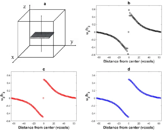
Let us consider a homogeneous material with isotropic elastic constants: Young’s modulus E=333.4 GPa and Poisson rationϑ=0.26. This approximately corresponds to the room temperature elastic constants of single crystalline Ni-based superalloys. The unit cell (Figure1a) is discretized in 128×128×128 voxels and contains a square-shaped inclusion discretized in 32×32×1 voxels corresponding to an Eshelby-like square prismatic loop perpendicular to thez-axis. In order to generate a shift of the upper surface of the inclusion relative to its lower surface by a Burgers vectorb(0, 0, b3), only the voxels within the inclusion are submitted to a non-zero eigenstrain tensor defined as:ε∗ij=0 exceptε33∗ =1. Then, we haveb3=t×ε∗33wheretthe thickness of the inclusion in thez-direction (i.e., the voxel size). This displacement field computed with the FFT algorithm using the different Green operators defined in Section2.1is represented alongz-axis in Figure1.
Materials 2018, 11, x FOR PEER REVIEW 4 of 12
discontinuity is approached. These oscillations (numerical artifacts) are not observed with the periodized operators 𝑩′ and 𝑩′′. An artificial damping of the oscillations in Figure 1b (such as a low pass filtering) might smooth these oscillations, but it would also smooth the discontinuity, which is not searched.
Figure 1. (a) Simulation of a square dislocation loop in plane (001) by a platelet with eigenstrain; (b) component 𝑢3 of the displacement field (normalized by 𝑏3) along the z axis (arrow) computed with the Green operator 𝑩 and showing spurious oscillations; (c) same component 𝑢3 computed with 𝑩′. The displacement at voxel (64,64,64) is zero in the center of the inclusion (c) and 𝑏3⁄2 on its surface; (d) same component 𝑢3 computed with 𝑩′′.
2.3. Voxelization Effect on the Displacement Field
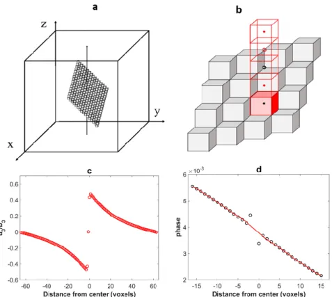
While the displacement field computed for dislocation loops having their planes parallel to the faces of the simulated volume is correctly given with discrete Green operators 𝑩′ or 𝑩′′, voxelization artifacts appear for inclined loops, as shown with 𝑩′ in Figure 2 for a dislocation loop with a [01̅1] Burgers vector lying in a (111) slip plane of a fcc crystal. The eigenstrain tensor is constrained in the region occupied by the dislocation loop (transformed voxels) and is given by:
𝜀𝑖𝑗∗ =𝐴𝑠
2𝑉(𝑛𝑖𝑏𝑗+ 𝑛𝑗𝑏𝑖) (6)
where 𝐴𝑠 is the area on which planes with normal 𝒏(𝑛1,𝑛2, 𝑛3) has slipped by a relative amount 𝒃(𝑏1,𝑏2, 𝑏3) and 𝑉 is the volume occupied by the dislocation loop [40,41]. As before, the dislocation loop is 32 voxels wide in the x and y directions, and 1 voxel thick but now with a z position such that 𝑥 + 𝑦 + 𝑧 = 𝑐𝑜𝑛𝑠𝑡𝑎𝑛𝑡. The displacement has been computed at the center of voxels with the periodized operator 𝑩′ along z (Figure 2b). As in Figure 1c, the displacement in the center of a voxel belonging to the loop plane (black dot in the reddish transformed voxel in Figure 2b) is zero. The displacement in the first neighboring voxels (red dot in Figure 2b) are shifted relative to the expected position, so that the displacement difference between these voxels is significantly lower than b, see Figure 2c. It can be checked in Figure 2b that each of these voxels shares three faces with a transformed voxel. A more detailed analysis shows that the second neighbors (which share three edges with transformed voxels) are also slightly shifted in the opposite direction. The result is shown in Figure 2d with: a strong localized oscillation of the phase (taken here as the displacement modulo b).
Figure 1. (a) Simulation of a square dislocation loop in plane (001) by a platelet with eigenstrain;
(b) componentu3of the displacement field (normalized byb3) along thezaxis (arrow) computed with the Green operatorBand showing spurious oscillations; (c) same componentu3computed withB0. The displacement at voxel (64,64,64) is zero in the center of the inclusion (c) andb3/2 on its surface;
(d) same componentu3computed withB00.
Materials2018,11, 1669 5 of 14
When computed along a line crossing a dislocation loop, the displacement field exhibits a discontinuity with a jump equal to Burgers vector b. This is indeed observed in Figure 1.
However, the displacement field computed with the usual Green operatorB(Figure1b) also shows spurious oscillations as soon as the discontinuity is approached. These oscillations (numerical artifacts) are not observed with the periodized operatorsB0andB00. An artificial damping of the oscillations in Figure1b (such as a low pass filtering) might smooth these oscillations, but it would also smooth the discontinuity, which is not searched.
2.3. Voxelization Effect on the Displacement Field
While the displacement field computed for dislocation loops having their planes parallel to the faces of the simulated volume is correctly given with discrete Green operatorsB0orB00, voxelization artifacts appear for inclined loops, as shown withB0in Figure2for a dislocation loop with a
011 Burgers vector lying in a(111)slip plane of a fcc crystal. The eigenstrain tensor is constrained in the region occupied by the dislocation loop (transformed voxels) and is given by:
ε∗ij = As
2V nibj+njbi
(6) where As is the area on which planes with normal n(n1,n2,n3) has slipped by a relative amount b(b1,b2,b3)andVis the volume occupied by the dislocation loop [40,41]. As before, the dislocation loop is 32 voxels wide in thexandydirections, and 1 voxel thick but now with a z position such that x+y+z=constant. The displacement has been computed at the center of voxels with the periodized operatorB0alongz(Figure2b). As in Figure1c, the displacement in the center of a voxel belonging to the loop plane (black dot in the reddish transformed voxel in Figure2b) is zero. The displacement in the first neighboring voxels (red dot in Figure2b) are shifted relative to the expected position, so that the displacement difference between these voxels is significantly lower thanb, see Figure2c. It can be checked in Figure2b that each of these voxels shares three faces with a transformed voxel. A more detailed analysis shows that the second neighbors (which share three edges with transformed voxels) are also slightly shifted in the opposite direction. The result is shown in Figure2d with: a strong localized oscillation of the phase (taken here as the displacement modulob).
Although the amplitude of this shift is small (less than 10% of the Burgers vector) it has unwanted consequences on the diffraction peak simulation:
The dislocation loops are surrounded by four impaired layers of voxels: As the scattered X-ray amplitude is proportional to the Fourier transform ofG·u(see Equation (8) in Section4), we can expect a phantom streak in the intensity in a direction perpendicular to the loop plane.
The displacement field near the edges of the loop (near the dislocation line) will be quite different from its expected value, and the strain field will not vary with the distancerto the dislocation line as 1/r. This will strongly affect the tails of the diffraction peaks.
Materials2018,11, 1669 6 of 14
Materials 2018, 11, x FOR PEER REVIEW 5 of 12
Although the amplitude of this shift is small (less than 10% of the Burgers vector) it has unwanted consequences on the diffraction peak simulation:
The dislocation loops are surrounded by four impaired layers of voxels: As the scattered X-ray amplitude is proportional to the Fourier transform of G·u (see Equation (8) in Section 4), we can expect a phantom streak in the intensity in a direction perpendicular to the loop plane.
The displacement field near the edges of the loop (near the dislocation line) will be quite different from its expected value, and the strain field will not vary with the distance 𝑟 to the dislocation line as 1 𝑟⁄ . This will strongly affect the tails of the diffraction peaks.
Figure 2. (a) Modeling of a dislocation loop in a (111) plane as a layer of voxels with eigenstrain; (b) position of the computed points relative to the transformed voxels with eigenstrains; (c) plot of the displacement field 𝑢3 (normalized by 𝑏3) along the z direction for the dislocation loop of Figure 2;
(d) local oscillation of the phase due to the voxelization of the dislocation loop (the representation is made for 32 voxels centered in the unit cell along z direction). The red line is approximately equal to the phase expected for this displacement field.
3. Sub-Voxelization Method to Correct Voxelization Artifacts
3.1. Sub-Voxelization Method
The (conceptually) simplest way to remove this voxelization artifact would be to work on a multiple grid (to multiply the number of voxels along each direction by 2, 4, or more), then to downsample the displacement field data. In that case, FFT algorithms would lose much of their interest due to these more demanding computational efforts. We show below that this can be done in a more “economical”—and simple—way by applying a patch to the FFT-computed displacement field. The basic method is to compute, on the same grid, the difference vector:
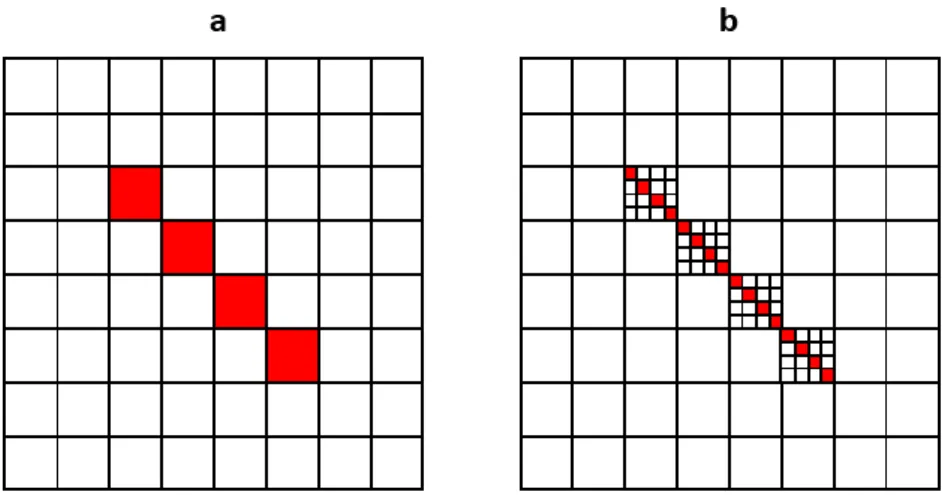
∆𝑖(𝒙) = 𝑢𝑖𝑠𝑢𝑏(𝒙) − 𝑢𝑖ℎ𝑜𝑚(𝒙) (7) where 𝑢𝑖𝑠𝑢𝑏(𝒙) is the displacement vector calculated for voxels where this eigenstrain is concentrated on a single plane of sub voxels (Figure 3b) and 𝑢𝑖ℎ𝑜𝑚 the displacement field in direction i of voxels with a uniform eigenstrain (Figure 3a). For the sake of clarity, we use 2D diagrams in Figure 3, but here the technique is applied to real 3D problems.
Figure 2. (a) Modeling of a dislocation loop in a (111) plane as a layer of voxels with eigenstrain;
(b) position of the computed points relative to the transformed voxels with eigenstrains; (c) plot of the displacement fieldu3(normalized byb3) along thezdirection for the dislocation loop of Figure2;
(d) local oscillation of the phase due to the voxelization of the dislocation loop (the representation is made for 32 voxels centered in the unit cell alongzdirection). The red line is approximately equal to the phase expected for this displacement field.
3. Sub-Voxelization Method to Correct Voxelization Artifacts
3.1. Sub-Voxelization Method
The (conceptually) simplest way to remove this voxelization artifact would be to work on a multiple grid (to multiply the number of voxels along each direction by 2, 4, or more), then to downsample the displacement field data. In that case, FFT algorithms would lose much of their interest due to these more demanding computational efforts. We show below that this can be done in a more “economical”—and simple—way by applying a patch to the FFT-computed displacement field.
The basic method is to compute, on the same grid, the difference vector:
∆i(x) =uisub(x)−uhomi (x) (7) whereusubi (x)is the displacement vector calculated for voxels where this eigenstrain is concentrated on a single plane of sub voxels (Figure3b) anduihomthe displacement field in directioniof voxels with a uniform eigenstrain (Figure3a). For the sake of clarity, we use 2D diagrams in Figure3, but here the technique is applied to real 3D problems.
Materials2018,11, 1669 7 of 14
Materials 2018, 11, x FOR PEER REVIEW 6 of 12
Figure 3. 2D representation of a dislocation loop in a tilted plane on a (8 × 8) fast Fourier transform (FFT) grid: (a) with a homogeneous eigenstrain 𝜺∗ in the voxels occupied by the dislocation loop; (b) with each voxel subdivided into 4 × 4 sub-voxels, only 4 of which have a 4 𝜺∗ eigenstrain field.
In order to compute the displacement due to sub-voxels, we use a 𝑁 × 𝑁 (𝑁 × 𝑁 × 𝑁) grid for 2D (resp.
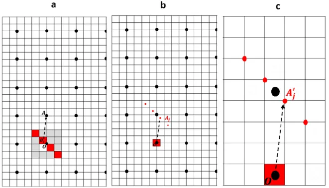
3D) problems where each voxel can be subdivided into 𝑛 × 𝑛 (𝑛 × 𝑛 × 𝑛) sub voxels. Only n (𝑛 × 𝑛) sub voxels are submitted to an eigenstrain field. At a point 𝑨 of the grid (black dots, Figure 4a), we need to compute the sum of the displacements 𝒖𝒊𝒋 due to the n (𝑛 × 𝑛) sub voxels j (center 𝑩𝒋) within a voxel centered at point 𝑶.
This sum is equivalent to the sum of the displacements due to a strained sub voxel at point 𝑶 on the grid points 𝑨𝒋 such as 𝑶𝑨𝒋= 𝑩𝒋𝑨 (Figure 4b). It is also equivalent to the sum of the displacements 𝒖′𝒊𝒋 due to a full voxel at point 𝑶 on the initial grid on points 𝑨′𝒋 such as 𝑶𝑨′𝒋= 𝑛𝑩𝒋𝑨 (Figure 4c). The only difference between these last two sums is due to the long-range strain field, and approximately results in a linear drift of the displacement.
As the end of the vectors 𝑶𝑨′𝒋 does not lie on the grid points (voxel centers) but on the corners of the voxels, the 𝒖′𝒊𝒋 displacements must be calculated with the shifted operator 𝑩′′ (Equation (5)). A last point is the scaling of the 𝒖𝒊𝒋 and 𝒖′𝒊𝒋 sums during the operations of Figure 4. To keep the one Burgers vector jump between both sides of the sub voxels plane in Figure 4a, the eigenstrain in the sub voxels must be multiplied by n. The backwards change of scale requires a division by n: there is no scaling factor between 𝑢𝑖ℎ𝑜𝑚 and 𝑢𝑖𝑠𝑢𝑏= ∑ 𝑢′𝑖𝑗.
Figure 4. (a) 2D representation of the computational grid. The black dots correspond to the voxels centers. A voxel with center O is discretized in 4 × 4 in 2D (4 × 4 × 4 in 3D) sub-voxels. The red sub- voxels have a non-zero eigenstrain. We want to compute the displacement field at point A, due to Figure 3.2D representation of a dislocation loop in a tilted plane on a (8×8) fast Fourier transform (FFT) grid: (a) with a homogeneous eigenstrainε∗ in the voxels occupied by the dislocation loop;
(b) with each voxel subdivided into 4×4 sub-voxels, only 4 of which have a 4ε∗eigenstrain field.
In order to compute the displacement due to sub-voxels, we use aN×N(N×N×N) grid for 2D (resp. 3D) problems where each voxel can be subdivided inton×n(n×n×n) sub voxels. Onlyn (n×n) sub voxels are submitted to an eigenstrain field. At a pointAof the grid (black dots, Figure4a), we need to compute the sum of the displacementsujidue to then(n×n) sub voxelsj(centerBj) within a voxel centered at pointO. This sum is equivalent to the sum of the displacements due to a strained sub voxel at pointOon the grid pointsAjsuch asOAj=BjA(Figure4b). It is also equivalent to the sum of the displacementsu0jidue to afullvoxel at pointOon the initial grid on pointsA0jsuch asOA0j
=nBjA(Figure4c). The only difference between these last two sums is due to the long-range strain field, and approximately results in a linear drift of the displacement. As the end of the vectorsOA0j
does not lie on the grid points (voxel centers) but on the corners of the voxels, theu0jidisplacements must be calculated with the shifted operatorB00(Equation (5)). A last point is the scaling of theuji andu0jisums during the operations of Figure4. To keep the one Burgers vector jump between both sides of the sub voxels plane in Figure4a, the eigenstrain in the sub voxels must be multiplied byn.
The backwards change of scale requires a division byn: there is no scaling factor betweenuhomi and usubi =∑u0ij.
Materials2018,11, 1669 8 of 14
Materials 2018, 11, x FOR PEER REVIEW 6 of 12
Figure 3. 2D representation of a dislocation loop in a tilted plane on a (8 × 8) fast Fourier transform (FFT) grid: (a) with a homogeneous eigenstrain 𝜺∗ in the voxels occupied by the dislocation loop; (b) with each voxel subdivided into 4 × 4 sub-voxels, only 4 of which have a 4 𝜺∗ eigenstrain field.
In order to compute the displacement due to sub-voxels, we use a 𝑁 × 𝑁 (𝑁 × 𝑁 × 𝑁) grid for 2D (resp.
3D) problems where each voxel can be subdivided into 𝑛 × 𝑛 (𝑛 × 𝑛 × 𝑛) sub voxels. Only n (𝑛 × 𝑛) sub voxels are submitted to an eigenstrain field. At a point 𝑨 of the grid (black dots, Figure 4a), we need to compute the sum of the displacements 𝒖𝒊𝒋 due to the n (𝑛 × 𝑛) sub voxels j (center 𝑩𝒋) within a voxel centered at point 𝑶.
This sum is equivalent to the sum of the displacements due to a strained sub voxel at point 𝑶 on the grid points 𝑨𝒋 such as 𝑶𝑨𝒋= 𝑩𝒋𝑨 (Figure 4b). It is also equivalent to the sum of the displacements 𝒖′𝒊𝒋 due to a full voxel at point 𝑶 on the initial grid on points 𝑨′𝒋 such as 𝑶𝑨′𝒋= 𝑛𝑩𝒋𝑨 (Figure 4c). The only difference between these last two sums is due to the long-range strain field, and approximately results in a linear drift of the displacement.
As the end of the vectors 𝑶𝑨′𝒋 does not lie on the grid points (voxel centers) but on the corners of the voxels, the 𝒖′𝒊𝒋 displacements must be calculated with the shifted operator 𝑩′′ (Equation (5)). A last point is the scaling of the 𝒖𝒊𝒋 and 𝒖′𝒊𝒋 sums during the operations of Figure 4. To keep the one Burgers vector jump between both sides of the sub voxels plane in Figure 4a, the eigenstrain in the sub voxels must be multiplied by n. The backwards change of scale requires a division by n: there is no scaling factor between 𝑢𝑖ℎ𝑜𝑚
and 𝑢𝑖𝑠𝑢𝑏= ∑ 𝑢′𝑖𝑗.
Figure 4. (a) 2D representation of the computational grid. The black dots correspond to the voxels centers. A voxel with center O is discretized in 4 × 4 in 2D (4 × 4 × 4 in 3D) sub-voxels. The red sub- voxels have a non-zero eigenstrain. We want to compute the displacement field at point A, due to Figure 4.(a) 2D representation of the computational grid. The black dots correspond to the voxels centers. A voxel with center O is discretized in 4×4 in 2D (4×4×4 in 3D) sub-voxels. The red sub-voxels have a non-zero eigenstrain. We want to compute the displacement field at point A, due to these deformed sub-voxels centered atBj. (b) Displacement field generated by a deformed sub-voxel centered at O on a row of sub-voxels centered atBjsuch asOAj=BjA. The sum of these displacements is equal to the previous displacement field. (c) Displacement field generated by a deformed voxel centered at O on a row of voxels (computed at the cornersA0jusing Green operatorB00) such asOA0j
=nBjA. This sum is equal to the previous sum.
We need to compute∆ij_pl(x)the difference in displacement in directionidue to a voxel which belongs to the plane “pl” (for fcc “pl” is equal to(111), 111
, 111 , 111
) of a dislocation loop with a Burgers vectorjat a position x relative to the transformed voxel. In practice, in a material with cubic symmetry, it is sufficient to compute∆13_(111)(x)and∆33_(111)(x), and to use the symmetries of the cube (fourfold [001] axis, threefold [111] axis, and 110
symmetry plane) (and suitable exchanges of the components ofx) to obtain the required components. As can be seen in Figure2b, ∆ij_pl(x) is non-zero only for the neighbors of the transformed voxel, except the drift due to the long range strain alluded above. The final computational procedure to determine∆ij_pl(x)and use the patch is now detailed:
Compute the fieldc0 : ε∗ defined in Equation (1) for an isolated voxel with the eigenstrain associated to a dislocation loop (Equation (6)) with a Burgers vector [001] in a (111) plane (see Figure2).
Compute the displacement field in directionsx(uhom1 ) andz(uhom3 ) at the voxels’ center around the transformed voxel by convolution with the discrete periodized operatorB0(Equation (4)).
Compute the displacement field in directionsxandzat the voxels’ corners around the transformed voxel by convolution with the shifted operatorB00 (Equation (5)).
Calculate theusub1 =∑u0j1andusub3 =∑u0j3sums (n×nterms for each sum) as in Figure4c, then the raw∆13_(111)(x)and∆33_(111)(x)for(x1,x2,x3)going from−3 to 3 times the voxel sizet.
Use the farthest voxels to correct the drift of the components so that all terms for largexare zero, and keep non zero only the terms for the first three neighbors.
The patch can then be applied on the raw (FFT-based) displacement field by adding the convolution of all transformed voxels of the different slip systems by the relevant∆ij_pl(x).
Materials2018,11, 1669 9 of 14
3.2. Results
For numerical tests, we used the same 128×128×128 grid as before, and the transformed voxel was divided into 8×8×8 sub voxels (using a reference medium with the same elastic constants as before). Only the final values in units of b (after drift correction) of∆13_(111)(x)and∆33_(111)(x)are used and other components are obtained by symmetries (AppendixA).
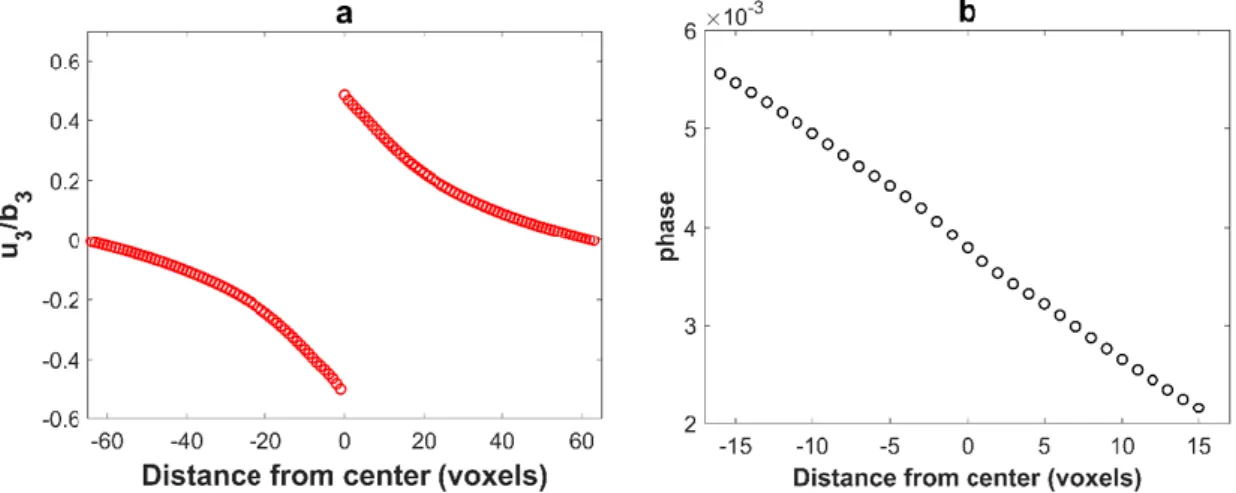
The patch was used on the same configuration as in Figure2. Figure 5a shows the resulting displacement field and Figure5b the phase (i.e., the displacement modulo a Burgers vector) in Burgers vector units. As it can be observed from Figure5a, the voxelization artifacts of the displacement field are removed thanks to the sub-voxelization method. In addition, the resulting phase varies smoothly even during the crossing of the dislocation loop which is more realistic, see Figure5b.
Materials 2018, 11, x FOR PEER REVIEW 7 of 12
these deformed sub-voxels centered at 𝐵𝑗. (b) Displacement field generated by a deformed sub-voxel centered at O on a row of sub-voxels centered at 𝐵𝑗 such as 𝑶𝑨𝒋= 𝑩𝒋𝑨. The sum of these displacements is equal to the previous displacement field. (c) Displacement field generated by a deformed voxel centered at O on a row of voxels (computed at the corners 𝑨′𝒋 using Green operator 𝑩′′) such as 𝑶𝑨′𝒋= 𝑛𝑩𝒋𝑨. This sum is equal to the previous sum.
We need to compute ∆𝑖𝑗_𝑝𝑙(𝒙) the difference in displacement in direction i due to a voxel which belongs to the plane “pl” (for fcc “pl” is equal to (111), (1̅11), (11̅1), (111̅)) of a dislocation loop with a Burgers vector j at a position x relative to the transformed voxel. In practice, in a material with cubic symmetry, it is sufficient to compute ∆13_(111)(𝒙) and ∆33_(111)(𝒙), and to use the symmetries of the cube (fourfold [001] axis, threefold [111]
axis, and (11̅0) symmetry plane) (and suitable exchanges of the components of 𝒙) to obtain the required components. As can be seen in Figure 2b, ∆𝑖𝑗_𝑝𝑙(𝒙) is non-zero only for the neighbors of the transformed voxel, except the drift due to the long range strain alluded above. The final computational procedure to determine
∆𝑖𝑗_𝑝𝑙(𝒙) and use the patch is now detailed:
Compute the field 𝒄𝟎: 𝜺∗ defined in Equation (1) for an isolated voxel with the eigenstrain associated to a dislocation loop (Equation (6)) with a Burgers vector [001] in a (111) plane (see Figure 2).
Compute the displacement field in directions x (𝒖𝟏𝒉𝒐𝒎) and z (𝒖𝟑𝒉𝒐𝒎) at the voxels’ center around the transformed voxel by convolution with the discrete periodized operator 𝑩′ (Equation (4)).
Compute the displacement field in directions x and z at the voxels’ corners around the transformed voxel by convolution with the shifted operator 𝑩′′ (Equation (5)).
Calculate the 𝒖𝟏𝒔𝒖𝒃= ∑ 𝒖′𝟏𝒋 and 𝒖𝟑𝒔𝒖𝒃= ∑ 𝒖′𝟑𝒋 sums (𝑛 × 𝑛 terms for each sum) as in Figure 4c, then the raw ∆13_(111)(𝒙) and ∆33_(111)(𝒙) for (𝑥1, 𝑥2, 𝑥3) going from −3 to 3 times the voxel size t.
Use the farthest voxels to correct the drift of the components so that all terms for large 𝒙 are zero, and keep non zero only the terms for the first three neighbors.
The patch can then be applied on the raw (FFT-based) displacement field by adding the convolution of all transformed voxels of the different slip systems by the relevant ∆𝑖𝑗_𝑝𝑙(𝒙).
3.2. Results
For numerical tests, we used the same 128 × 128 × 128 grid as before, and the transformed voxel was divided into 8 × 8 × 8 sub voxels (using a reference medium with the same elastic constants as before). Only the final values in units of b (after drift correction) of ∆13_(111)(𝒙) and ∆33_(111)(𝒙) are used and other components are obtained by symmetries (Appendix A).
The patch was used on the same configuration as in Figure 2. Figure 5a shows the resulting displacement field and Figure 5b the phase (i.e., the displacement modulo a Burgers vector) in Burgers vector units. As it can be observed from Figure 5a, the voxelization artifacts of the displacement field are removed thanks to the sub- voxelization method. In addition, the resulting phase varies smoothly even during the crossing of the dislocation loop which is more realistic, see Figure 5b.
Figure 5. (a) Plot of the displacement field 𝑢3 (normalized by 𝑏3) along the z direction for dislocation loop illustrated on Figure 2. The voxelization artifacts are removed by the sub-voxel method described Figure 5.(a) Plot of the displacement fieldu3(normalized byb3) along thezdirection for dislocation loop illustrated on Figure2. The voxelization artifacts are removed by the sub-voxel method described above. (b) The phase (i.e., the displacement modulo a Burgers vector). With this correction, the phase is almost continuous.
4. Application on Diffraction Peak Simulation
In this section, we show simulated diffraction peaks in order to point the effects of voxelization artifacts and of the patch on numerical results. Under kinematical conditions and assuming a coherent beam, the amplitude of a diffracted wave at a positionqin the vicinity of a reciprocalGlattice vector is [14,18,42–44]:
A(q) =FT[A0(x)×F(G,x)×exp(−2iπG·u(x))] (8) wherexis the position of the scattering atom,A0(x)is the amplitude of the incidence wave,F(G,x) is the local structure factor, andu(x)the displacement field. The scattered intensity isI(q)=|A(q)|2. For a face-centered cubic crystal, this intensity is non zero whenG(h,k,l) is such ash,k, andlhave the same parity. Here two diffraction vectorsG(200) andG(002) are used. They respectively correspond toG·b= 0 andG·b= 1. The 3D diffracted intensity has been calculated using the FFT instead of the continuous Fourier transform, then summed in the planes perpendicular to theGvector to obtain a linear plot alongGequivalent to aI(2θ) plot. In Figure6a (G(200)) and Figure6c (G(002)), we show the diffracted intensity (logarithmic scale) as a function of the pixel positioni, and in Figure6b,d a logarithmic/logarithmic plot of the intensity vs.|i−i0|wherei0is the center of the peak. In order to only study the effect of the displacement fields, we set A0(x) =1 andF(G,x) =1 for these simulations.
Materials2018,11, 1669 10 of 14
Materials 2018, 11, x FOR PEER REVIEW 8 of 12
above. (b) The phase (i.e., the displacement modulo a Burgers vector). With this correction, the phase is almost continuous.
4. Application on Diffraction Peak Simulation
In this section, we show simulated diffraction peaks in order to point the effects of voxelization artifacts and of the patch on numerical results. Under kinematical conditions and assuming a coherent beam, the amplitude of a diffracted wave at a position 𝒒 in the vicinity of a reciprocal 𝑮 lattice vector is [14,18,42–44]:
𝐴(𝒒) = 𝐹𝑇[𝐴0(𝒙) × 𝐹(𝑮, 𝒙) × 𝑒𝑥𝑝 (−2𝑖𝜋 𝑮 ∙ 𝒖(𝒙))] (8) where 𝒙 is the position of the scattering atom, 𝐴0(𝒙) is the amplitude of the incidence wave, 𝐹(𝑮, 𝒙) is the local structure factor, and 𝒖(𝒙) the displacement field. The scattered intensity is 𝐼(𝒒)= |𝐴(𝒒)|2. For a face-centered cubic crystal, this intensity is non zero when G (h, k, l) is such as h, k, and l have the same parity. Here two diffraction vectors G (200) and G (002) are used. They respectively correspond to G∙b = 0 and G∙b = 1. The 3D diffracted intensity has been calculated using the FFT instead of the continuous Fourier transform, then summed in the planes perpendicular to the G vector to obtain a linear plot along G equivalent to a I(2θ) plot. In Figure 6a (G (200)) and 6c (G (002)), we show the diffracted intensity (logarithmic scale) as a function of the pixel position 𝑖, and in figures 6b and 6d a logarithmic/logarithmic plot of the intensity vs. |𝑖 − 𝑖0| where 𝑖0 is the center of the peak. In order to only study the effect of the displacement fields, we set A0(𝒙) = 1 and 𝐹(𝑮, 𝒙) = 1 for these simulations.
Figure 6. Simulated diffracted intensity as a function of the pixel position (logarithmic scale). 3D configuration is represented in a 1D plot by making the sum in each plane along an x-axis. Different way for computing the displacement fields are studied for a dislocation loop with a 𝑎2[01̅1] Burgers vector lying in a (111) slip plane. (a) Diffracted vector studied is G (200) corresponding to G∙b = 0.
(b) Log/log representation of the intensity vs. |𝑖 − 𝑖0|. (c) and (d) same as (a) et (b) but the studied diffracted vector is G (002) (G∙b = 1).
Figure 6. Simulated diffracted intensity as a function of the pixel position (logarithmic scale).
3D configuration is represented in a 1D plot by making the sum in each plane along anx-axis.
Different way for computing the displacement fields are studied for a dislocation loop with a2a 011 Burgers vector lying in a(111)slip plane. (a) Diffracted vector studied isG (200) corresponding toG·b= 0. (b) Log/log representation of the intensity vs.|i−i0|. (c) and (d) same as (a) et (b) but the studied diffracted vector isG(002) (G·b= 1).
The peak shape near the top of the peaks is the same for both computing methods. It is perfectly symmetric in theG·b= 0 case and exhibits a bump on the right side forG·b= 1. The long-range behavior is, however, quite different. When the displacement field has been calculated with the usual truncated operator (black line), a phantom peak is observed at large|i−i0|(at largeq), which is due to the short period oscillations near the displacement field discontinuity (Figure1a). The behavior of the peak calculated with the modified Green operator (red curve) is only slightly better: the intensity at large q is underestimated in one case and overestimated in the other. When the intensity has been calculated with the sub voxel patch (dark blue curve) the long range intensity follows the expectedI0|i−i0|−3 law [45,46]: the peak tails are indeed related to the highly distorted zones near the dislocations’ cores.
However, the dark blue curve saturates at very largeq. We suppose this is due to the use of the FFT instead of the continuous Fourier transform in the calculation of the scattered amplitude (Equation (8)).
The plot of Figure6represents only one period in Fourier space, and is repeated over and over on all Fourier space. We can now calculate the intensity of the tails of these repetitions:
Ineib.=
∑
I0|i−i0−128m|−3 (9)where m varies from−5 to 5 (zero excluded). If we now plot the difference between the dark blue intensity curve and this background line, we obtain the pink curve. On the log./log. plots, Figure6b,d, it can be checked that this curve follows theI0|i−i0|−3law to the end. Thus, the residual error in the
Materials2018,11, 1669 11 of 14
intensity computed by FFT results of the FFT itself, and not from an error on the sub voxel-corrected displacement field. If the number of voxels is increased to 5123or 10243while keeping the physical size of the representative volume constant, this residual error should fall down to undetectable levels.
5. Conclusions
In this paper, we have shown that although the use of a periodized Green operator in the FFT-based method improves the final displacement field solution in a representative volume containing discontinuities (dislocation loops), artifacts due to the voxelization of the dislocation loop planes are still present with respect to analytical solutions. These artifacts have unwanted consequences on the tails of diffraction peaks simulated by using this displacement field as input data.
We have introduced a patch through a sub-voxelization method, which corrects these artifacts by simulating the displacement field without employing a finer grid resolution. A simple construction method for this patch has been given and the patch can be used in a single post-processing step to modify the initial FFT-based displacement field.
The modified displacement field has been used to simulate one-dimensional diffraction peaks.
The procedure strongly improves the shape of the peaks’ tails, i.e., it gives a good description of the displacement field and the phase near the dislocation lines.
Author Contributions:For the present paper, K.E. performed the simulation work and wrote the first draft of the paper; A.J. analyzed numerical results and helped in the simulation; G.R. helped in constructing the computer code and in analyzing results; S.B. helped in developing the first theoretical part of the paper. The paper was written by K.E., A.J. and S.B.
Funding: This research was funded by the french National Research Agency (ANR), grant number ANR-11-LABX-0008-01 (LabEx DAMAS).
Acknowledgments:Gabor Ribarik greatly acknowledges the support of the Janos Bolyai Research Fellowship of the Hungarian Academy of Sciences.
Conflicts of Interest:The authors declare no conflict of interest.
Appendix A
∆33_(111)(x1,x2,x3) and ∆13_(111)(x1,x2,x3) have these symmetries due to the permutation properties of the plane(111):
∆33_(111)(x1,x2,x3) =∆33_(111)(x2,x1,x3)
∆33_(111)(x1,x2,x3) =−∆33_(111)(−x1,−x2,−x3)
∆13_(111)(x1,x2,x3) =−∆13_(111)(−x1,−x2,−x3)
The others values of ∆ij_(111)(x) are given as function of ∆33_(111)(x1,x2,x3) and
∆13_(111)(x1,x2,x3):
∆11_(111)(x1,x2,x3) =∆33_(111)(x3,x2,x1) ∆12_(111)(x1,x2,x3) =∆13_(111)(x1,x3,x3)
∆22_(111)(x1,x2,x3) =∆33_(111)(x1,x3,x2) ∆31_(111)(x1,x2,x3) =∆13_(111)(x3,x2,x1).
∆32_(111)(x1,x2,x3) =∆13_(111)(x3,x1,x2) ∆21_(111)(x1,x2,x3) =∆13_(111)(x1,x3,x2)
∆23_(111)(x1,x2,x3) =∆13_(111)(x2,x1,x3)
Materials2018,11, 1669 12 of 14
The value of∆33(x1,x2,x3)and∆13(x1,x2,x3)for the remaining plane 111 , 111
, 111 are obtained using these symmetries:
∆33_(111)(x1,x2,x3) =∆33_(111)(x2,−x1,x3)
∆13_(111)(x1,x2,x3) =∆13_(111)(−x1,x2,x3)
∆33_(111)(x1,x2,x3) =∆33_(111)(−x2,x1,x3)
∆13_(111)(x1,x2,x3) =∆13_(111)(x1,−x2,x3)
∆33_(111)(x1,x2,x3) =−∆33_(111)(x2,x1,−x3)
∆13_(111)(x1,x2,x3) =−∆13_(111)(x1,x2,−x3) References
1. Graverend, J.-B.L.; Dirand, L.; Jacques, A.; Cormier, J.; Ferry, O.; Schenk, T.; Gallerneau, F.; Kruch, S.;
Mendez, J. In Situ Measurement of theγ/γ0Lattice Mismatch Evolution of a Nickel-Based Single-Crystal Superalloy during Non-isothermal Very High-Temperature Creep Experiments.Metall. Mater. Trans. A2012, 43, 3946–3951. [CrossRef]
2. Robinson, I.; Harder, R. Coherent X-ray diffraction imaging of strain at the nanoscale.Nat. Mater.2009,8, 291–298. [CrossRef] [PubMed]
3. Pfeifer, M.A.; Williams, G.J.; Vartanyants, I.A.; Harder, R.; Robinson, I.K. Three-dimensional mapping of a deformation field inside a nanocrystal.Nature2006,442, 63. [CrossRef] [PubMed]
4. Ungár, T. Strain Broadening Caused by Dislocations. Available online:https://www.scientific.net/MSF.278- 281.151(accessed on 16 June 2018).
5. Ungár, T.; Gubicza, J.; Ribárik, G.; Borbély, A. Crystallite size distribution and dislocation structure determined by diffraction profile analysis: Principles and practical application to cubic and hexagonal crystals.J. Appl. Crystallogr.2001,34, 298–310. [CrossRef]
6. Ribárik, G.; Ungár, T.; Gubicza, J. MWP-fit: A program for multiple whole-profile fitting of diffraction peak profiles by ab initio theoretical functions.J. Appl. Crystallogr.2001,34, 669–676. [CrossRef]
7. Ribárik, G.; Gubicza, J.; Ungár, T. Correlation between strength and microstructure of ball-milled Al–Mg alloys determined by X-ray diffraction.Mater. Sci. Eng. A2004,387, 343–347. [CrossRef]
8. Balogh, L.; Ribárik, G.; Ungár, T. Stacking faults and twin boundaries in fcc crystals determined by X-ray diffraction profile analysis.J. Appl. Phys.2006,100, 023512. [CrossRef]
9. Groma, I. X-ray line broadening due to an inhomogeneous dislocation distribution.Phys. Rev. B1998,57, 7535. [CrossRef]
10. Tréhorel, R.; Ribarik, G.; Schenk, T.; Jacques, A. Real time study of transients during high temperature creep of a Ni-based superlloy by far field high energy synchrotron X-rays diffraction.J. Appl. Crystallogr.2018, under review.
11. Tréhorel, R.Comportement Mécanique Haute Température Du Superalliage Monocristallin Am1: Etude In-Situ Par Une Nouvelle Technique De Diffraction En Rayonnement Synchrotron; Universitéde Lorraine: Nancy, France, 2018.
12. Bernier, J.V.; Park, J.-S.; Pilchak, A.L.; Glavicic, M.G.; Miller, M.P. Measuring Stress Distributions in Ti-6Al-4V Using Synchrotron X-Ray Diffraction.Metall. Mater. Trans. A2008,39, 3120–3133. [CrossRef]
13. Miller, M.P.; Bernier, J.V.; Park, J.-S.; Kazimirov, A. Experimental measurement of lattice strain pole figures using synchrotron X rays.Rev. Sci. Instrum.2005,76, 113903. [CrossRef]
14. Jacques, A. From Modeling of Plasticity in Single-Crystal Superalloys to High-Resolution X-rays Three-Crystal Diffractometer Peaks Simulation.Metall. Mater. Trans. A2016,47, 5783–5797. [CrossRef]
15. Weisbrook, C.M.; Gopalaratnam, V.S.; Krawitz, A.D. Use of finite element modeling to interpret diffraction peak broadening from elastic strain distributions.Mater. Sci. Eng. A1995,201, 134–142. [CrossRef]
16. Miller, M.P.; Dawson, P.R. Understanding local deformation in metallic polycrystals using high energy X-rays and finite elements.Curr. Opin. Solid State Mater. Sci.2014,5, 286–299. [CrossRef]
17. Demir, E.; Park, J.-S.; Miller, M.P.; Dawson, P.R. A computational framework for evaluating residual stress distributions from diffraction-based lattice strain data.Comput. Methods Appl. Mech. Eng.2013,265, 120–135.
[CrossRef]
Materials2018,11, 1669 13 of 14
18. Vaxelaire, N.; Proudhon, H.; Labat, S.; Kirchlechner, C.; Keckes, J.; Jacques, V.; Ravy, S.; Forest, S.; Thomas, O.
Methodology for studying strain inhomogeneities in polycrystalline thin films during in situ thermal loading using coherent X-ray diffraction.New J. Phys.2010,12, 035018. [CrossRef]
19. Song, X.; Xie, M.; Hofmann, F.; Illston, T.; Connolley, T.; Reinhard, C.; Atwood, R.C.; Connor, L.;
Drakopoulos, M.; Frampton, L. Residual stresses and microstructure in powder bed direct laser deposition (PB DLD) samples.Int. J. Mater. Form.2015,8, 245–254. [CrossRef]
20. Hofmann, F.; Song, X.; Jun, T.-S.; Abbey, B.; Peel, M.; Daniels, J.; Honkimäki, V.; Korsunsky, A.M. High energy transmission micro-beam Laue synchrotron X-ray diffraction.Mater. Lett.2010,64, 1302–1305. [CrossRef]
21. Hofmann, F.; Abbey, B.; Liu, W.; Xu, R.; Usher, B.F.; Balaur, E.; Liu, Y. X-ray micro-beam characterization of lattice rotations and distortions due to an individual dislocation.Nat. Commun.2013,4, 2774. [CrossRef]
[PubMed]
22. Suter, R.M.; Hennessy, D.; Xiao, C.; Lienert, U. Forward modeling method for microstructure reconstruction using X-ray diffraction microscopy: Single-crystal verification.Rev. Sci. Instrum.2006,77, 123905. [CrossRef]
23. Moulinec, H.; Suquet, P. A numerical method for computing the overall response of nonlinear composites with complex microstructure.Comput. Methods Appl. Mech. Eng.1998,157, 69–94. [CrossRef]
24. Moulinec, H.; Suquet, P. Fast numerical method for computing the linear and nonlinear properties of composites.C. R. Acad. Sci. Ser. II1994,318, 1417–1423.
25. Michel, J.C.; Moulinec, H.; Suquet, P. A computational scheme for linear and non-linear composites with arbitrary phase contrast.Int. J. Numer. Methods Eng.2001,52, 139–160. [CrossRef]
26. Müller, W. Mathematical vs. Experimental Stress Analysis of Inhomogeneities in Solids.J. Phys. IV Colloq.
1996,6, C1-139–C1-148. [CrossRef]
27. Vinogradov, V.; Milton, G.W. An accelerated FFT algorithm for thermoelastic and non-linear composites.
Int. J. Numer. Methods Eng.2008,76, 1678–1695. [CrossRef]
28. Anglin, B.S.; Lebensohn, R.A.; Rollett, A.D. Validation of a numerical method based on Fast Fourier Transforms for heterogeneous thermoelastic materials by comparison with analytical solutions.
Comput. Mater. Sci.2014,87, 209–217. [CrossRef]
29. Graham, J.T.; Rollett, A.D.; LeSar, R. Fast Fourier transform discrete dislocation dynamics.Model. Simul.
Mater. Sci. Eng.2016,24, 085005. [CrossRef]
30. Berbenni, S.; Taupin, V.; Djaka, K.S.; Fressengeas, C. A numerical spectral approach for solving elasto-static field dislocation and g-disclination mechanics.Int. J. Solids Struct.2014,51, 4157–4175. [CrossRef]
31. Eyre, D.J.; Milton, G.W. A fast numerical scheme for computing the response of composites using grid refinement.Eur. Phys. J. AP1999,6, 41–47. [CrossRef]
32. Prakash, A.; Lebensohn, R.A. Simulation of micromechanical behavior of polycrystals: Finite elements versus fast Fourier transforms.Model. Simul. Mater. Sci. Eng.2009,17, 064010. [CrossRef]
33. Lebensohn, R.A. N-site modeling of a 3D viscoplastic polycrystal using Fast Fourier Transform.Acta Mater.
2001,49, 2723–2737. [CrossRef]
34. Lebensohn, R.A.; Rollett, A.D.; Suquet, P. Fast fourier transform-based modeling for the determination of micromechanical fields in polycrystals.JOM2011,63, 13–18. [CrossRef]
35. Lebensohn, R.A.; Kanjarla, A.K.; Eisenlohr, P. An elasto-viscoplastic formulation based on fast Fourier transforms for the prediction of micromechanical fields in polycrystalline materials.Int. J. Plast.2012,32–33, 59–69. [CrossRef]
36. Suquet, P.; Moulinec, H.; Castelnau, O.; Montagnat, M.; Lahellec, N.; Grennerat, F.; Duval, P.; Brenner, R.
Multi-scale modeling of the mechanical behavior of polycrystalline ice under transient creep.Procedia IUTAM 2012,3, 76–90. [CrossRef]
37. Eloh, K.S.; Jacques, A.; Berbenni, S. Development of a new consistent discrete Green operator for FFT-based methods to solve heterogeneous problems with eigenstrain.Int. J. Plast.2018. submitted.
38. Hirth, J.P.; Lothe, J. Theory of Dislocations; Krieger Publishing Company: Malabar, FL, USA, 1982;
ISBN 978-0-89464-617-1.
39. Mura, T. Micromechanics of Defects in Solids, 2nd ed.; Mechanics of Elastic and Inelastic Solids;
Springer: Dordrecht, The Netherlands, 1987; ISBN 978-90-247-3256-2.
40. Li, Q.; Anderson, P.M. A Compact Solution for the Stress Field from a Cuboidal Region with a Uniform Transformation Strain.J. Elast.2001,64, 237–245. [CrossRef]
Materials2018,11, 1669 14 of 14
41. Anderson, P.M. Crystal-based plasticity. InFundamentals of Metal Forming; Wagoner, R.H., Chenot, J.-L., Eds.;
Wiley: New York, NY, USA, 1997; pp. 263–293.
42. Takagi, S. A Dynamical Theory of Diffraction for a Distorted Crystal.J. Phys. Soc. Japan1969,26, 1239–1253.
[CrossRef]
43. Vartanyants, I.A.; Yefanov, O.M. Coherent X-ray Diffraction Imaging of Nanostructures. arXiv2013, arXiv:1304.5335.
44. Takagi, S. Dynamical theory of diffraction applicable to crystals with any kind of small distortion.
Acta Crystallogr.1962,15, 1311–1312. [CrossRef]
45. Ungár, T. Microstructural parameters from X-ray diffraction peak broadening.Scr. Mater.2004,51, 777–781.
[CrossRef]
46. Krivoglaz, M.A.Theory of X-Ray and Thermal Neutron Scattering by Real Crystals; Springer: New York, NY, USA, 1969; ISBN 978-1-4899-5584-5.
© 2018 by the authors. Licensee MDPI, Basel, Switzerland. This article is an open access article distributed under the terms and conditions of the Creative Commons Attribution (CC BY) license (http://creativecommons.org/licenses/by/4.0/).