CHAPTER TWENTY-ONE
COLLOIDS AND MACROMOLECULES
The twin topics of this chapter have vast extensions into applied areas, ranging from the behavior of detergents, emulsions, suspensions, and gels, to the proper- ties of synthetic and biological polymers. We will be dealing with particles small enough or molecules large enough that their size, shape, and interfacial properties play a major role in determining behavior. Particle-particle interactions may be of great importance; these will be of the van der Waals type, including hydrogen bonding. One of the very significant contributions of colloid chemistry to funda- mental science has been to the elucidation of the nature and manner of propaga- tion of such secondary interactions. Modern colloid chemistry is in fact far more interesting and important than the meaning of the word colloid—gluelike—
would imply!
The physical chemistry of macromolecules overlaps with that of colloidal sys- tems. There are many experimental techniques which are common to the two subjects. In addition, however, polymer chemistry is concerned with reaction kinetics and with the stereochemistry of the primary or chemical bonding of the molecule.
The plan of the chapter is as follows. We take up first the topic of lyophobic colloids—a more complex subject than might at first be imagined—then lyophilic colloids and an excursion into rheology. Because of the difficulty in covering the field in any really adequate way, only a few rather descriptive aspects of polymer chemistry are presented. We conclude with a Special Topics section on electro- kinetic phenomena, a part of surface chemistry not so far considered.
21-1 Lyophobic Colloids
The term "lyophobic" means solvent-hating, and the class of lyophobic colloids includes all dispersed systems in which the dispersed material is neither in true solution nor aggregated. A gold or silver iodide sol (a sol being a suspension of
899
solid particles in a liquid medium) is an example of a lyophobic system. The particles tend to stay separated from each other; they are not strongly solvated nor do they otherwise interact with the solvent, in contrast to gel-forming sub
stances. We consider here only one aspect of the subject, namely the theoretical explanation of why it is that lyophobic colloids are fundamentally unstable toward flocculation on the one hand, and why, on the other hand, the rate of flocculation may be very slow. As an example of this last point, some of Michael Faraday's gold sols—not yet flocculated—are still to be seen in the British Museum. There must evidently be present forces both of attraction and of repulsion.
The attraction is due to van der Waals forces, often mainly dispersion in type (see Section 8-ST-l), and the repulsion is due to the electric field around each particle. Both forces can be long-range, that is, extend over hundreds of angstroms.
Being quite general in nature, these forces play an important role in any nonideal condensed system, which, incidentally, means virtually all biological ones. The importance of lyophobic colloids is partly that their study has served as a means for the experimental characterization of long-range forces.
A. Long-Range Dispersion Forces
The dispersion attraction between two like atoms is given by Eq. (8-61), which we will write in the simplified form
€ ( * ) = - £ , (21-1) where A = %hv0oc2, α being the polarizability of the atom and hv0, its ionization
potential. This is a general force of attraction, largely independent of the chemical nature of the atom; it arises from small, mutually induced perturbations in the electron clouds and is additive (to a first approximation). A representative value of A would be 1 0- 6 0 erg cm6.
A consequence of the additive nature of dispersion interactions is that an atom near a large body of matter experiences a total attraction given by integrating Eq. (21-1) over the length, breadth, and depth of the body. For a semi-infinite
slab, the result is
€
C*)atom-slab = ~
> (21-2) where η is the number of atoms in the slab per cubic centimeter. To get the attractive force between two slabs, we must consider a column of atoms in the second one, as illustrated in Fig. 21-1, and integrate over its depth. The result for two infinitely thick slabs is
e
Wslab-slab =
Ϊ2π ~χ* 9 (21-3)where Η is called the Hamaker constant (alternatively given the symbol A), and is equal to π2η2Α. For two closely approaching spheres,
Φ 0 = - ^ £ τ , (21-4) where a is the radius and χ is the surface-to-surface distance, assumed to be small
21-2 LYOPHOBIC COLLOIDS 901
F I G . 2 1 - 1 . Van der Waals forces between a surface and a column of molecules. [From A. W.
Adamson, "Physical Chemistry of Surfaces," 3rd ed. Copyright 1976, Wiley (Interscience), New York. Used by permission of John Wiley & Sons, Inc.]
compared to a. A typical value for Η is about 10~1 3 erg. These interaction poten
tials are long-range in the sense that they fall off only slowly with distance, that is, as l/x2 or as l/x.
Consider t w o spherical colloidal particles of 1 μ ( 1 0- 4 c m ) radius, for which Η is 1 0- 1 3 erg, s o that f r o m Eq. (21-4) *(x) = — 1 0 " 16/x erg. A t 100 A or 1 0 "8 c m separation, c(x) is therefore
— 1 0- 1 2 erg. This is a small quantity, but much larger than the kinetic energy of the particles kT, which is 4 χ 1 0 ~1 4 erg at 25°C.
As the example demonstrates, once two colloidal particles are in each other's vicinity, either as a result of diffusion or of the action of convection currents, they should drift together and seize. The repulsive potential that prevents this is now discussed.
β. Electrostatic Repulsion. The Diffuse Double Layer
We consider first a single particle, large enough for its surface to be treated as flat, and having a surface charge σ0 per square centimeter and corresponding potential φ0 . The particle is in a liquid medium containing an electrolyte of con
centration n0 , which we take to be uni-univalent in type. We further assume ψ0 to be positive so that negative ions of the electrolyte are attracted to the surface and positive ions are repelled. The potential energy of an ion in a potential φ is just βφ, so by the Boltzmann principle the concentration of ions in a region near the surface is
n - = nQe'^kT, n+ - n0e~e^kT, (21-5)
where φ is the potential at some distance χ away from the surface. The net charge density at this point is then
βφ
ρ = e(n+ — η ) = — 2n0e sinh -^ψ (21-6)
[remembering that sinh χ = \(ex — e~x)]. The derivation is so far entirely anal-
ogous to that of the Debye-Huckel theory [compare Eq. (12-76)], and we proceed to invoke the Poisson equation (12-77), thus obtaining
V V = ^ s i n h | i [Eq. (12-78)], where D is the dielectric constant of the medium.
The derivation now takes a turn from the Debye-Huckel one since in the present case ν2φ is just ά2φ\άχ2 and Eq. (12-78) can be integrated directly. The result is somewhat complicated, but if βφ/kT (for ions of charge z, ζβφ/kT) is small com
pared to unity, one obtains the simple result
Φ = Ψ*β-«\ (21-7) where κ is the Debye-Huckel constant, defined for a uni-univalent electrolyte by
Eq. (12-80),
2 _ 8ττη0β2 DkT '
The potential thus decays exponentially with distance into the solution.
(21-8)
T h e behavior of Eq. (21-7) is illustrated in Fig. 21-2 for φ0 = 25 m V (1 m V = 0.001 V ) ; for a singly charged ion the corresponding potential energy is 23 cal m o l e- 1; 25 mV therefore corre
sponds to about kTat 25°C. Notice that the range of φ is about 1 0 0 A for fairly typical electrolyte concentrations, and that φ drops off more rapidly the higher the concentration and the higher the valence of the electrolyte ions.
The physical situation is that for a surface of potential φ0 ; the nearby solution has an excess of negative over positive ions, or a net charge density ρ which, along with φ, diminishes approximately exponentially with distance. The system as a whole is electrically neutral, so that the surface of the solid must have a surface
21-2 LYOPHOBIC COLLOIDS 903
The picture is one of a positively charged surface and a counterbalancing net excess of negative charge in the neighboring solution. This last is diffuse, and the system is called a diffuse double layer. The potential φ has decayed to l/e of φ0 at a distance l/κ, and consequently the electrical "center of gravity" of charge in the solution may be regarded as located at a distance l/#c from the surface. In the case of the Debye-Huckel theory, Ι/κ is the radius of the ionic atmosphere.
If two charged surfaces, such as those of two colloidal particles, approach, the repulsion depends on the value of φ at the midpoint. The derivation will not be given here [see Adamson (1976)] but only an approximate result:
€(x) = 6 4 n»k T (21-10)
where γ = (eVf>i2 — l)/(ey°/2 + 1), y0 = ζβφ0/ΙίΤ, n0 is in molecules per cubic centimeter, and e(x) is the repulsion potential in ergs per square centimeter.
Suppose that y0 = 1, χ = 1 0- ec m , and the concentration of uni-univalent electrolyte is 0.001 M, s o that κ is a b o u t 1 0e c m "1 (and KX = 1). W e obtain
64(0.001)(10-3)6.02 χ \023 kT / 1.65 - 1 \" „ „ „ < Λ„ ,
€(x) = — 0.135 = 3.13 χ 1 01 1 kT erg c m "2. 106 \ 1.65 + 1 /
C. Flocculation of Colloidal Suspensions
The flocculation or coming together of colloidal particles can be examined in the light of the preceding estimates of the attraction and repulsion potentials. The
F I G . 2 1 - 3 . The diffuse double layer as equivalent to a plane of excess charge in solution at distance 1 /* from a surface of equal but opposite charge.
charge density as illustrated in Fig. 21-3,
« 0.5 x 1 0- 1 2
Έ \0kT oo
-ΙΟΑτΓ - 0 . 5 χ 1 0- · 2
1.5 x 1 0- 1 2
1 χ 1 0- 1 2
- 2 0 kT 30 kT
20 kT
1 kT
2 3.5
F I G . 21-4. The effect of electrolyte concentration on the interaction potential energy between two spheres. (From E. J. W. Verwey and J. Th. G. Overbeek, "Theory of Lyophobic Colloids."
Elsevier, Amsterdam, 1948.)
approximate net potential is given by the sum of Eq. (21-3) or Eq. (21-4) and Eq. (21-8),
The function *(x) is illustrated in Fig. 21-4. We assume particles of radius about 1 0 "5 cm or area about 3 X 1 0 "1 0 c m2 in applying Eq. (21-3). At small κ or low electrolyte concentration the electrostatic repulsion is strong and the colloidal particles will be virtually unable to approach each other; the suspension should be relatively stable. The barrier diminishes with increasing electrolyte concentration and eventually disappears.
One may, in fact, calculate the critical electrolyte concentration such that the barrier is just zero from the condition that e(x) = 0 and de(x)/dx = 0. The result
ing equation gives n0(c r i t) as proportional to 1/z6. Thus for a z-z electrolyte, equiv
alent conditions with respect to producing flocculation should be in the order 1 : (έ)6: (έ)6 or 100 : 1.6 :0.13 for 1-1, 2-2, and 3-3 electrolytes, respectively. This is essentially the experimental observation as embodied in what is known as the Schulze-Hardy rule.
Another factor, not explicitly mentioned so far, is that while ψ0 reflects the intrinsic nature of the particle-medium interface, it may be modified by adsorbed ions. The potential of colloidal Agl particles is, for example, very dependent on the concentration of Ag+ or I- ions in the solution and in general would be affected
€(*) (21-11),
21-2 ASSOCIATION COLLOIDS. COLLOIDAL ELECTROLYTES 905 by the presence of any other adsorbable ions. One may thus vary φ0 as well as electrolyte concentration, and studies of this type have allowed approximate experimental values of the Hamaker constant Η to be calculated from flocculation rates.
The basis of the calculation is that the flocculation rate should be just the encounter rate given by Eq. (15-26) modified by the factor exp(—€*/&Γ), where
€* is the height of the barrier (such as shown in Fig. 21-4). Thus e* may be cal
culated from the measured flocculation rate and, by means of Eq. (21-11), related to H.
It should be mentioned that Η has been measured directly as a weak force of attraction between a spherical surface and a plate. The force is very small, of the order of 0.01 dyn for a separation of about 1 0- 4 cm and the required apparatus is quite ingenious in design—the measurements come from the laboratories of J. Th. Overbeek in Holland and Β. V. Derjaguin in the USSR. It is quite a triumph that the approximate wave mechanical theory, the direct measurements, and the indirect calculation through flocculation rates agree in value of Η to within at least an order of magnitude.
21-2 Association Colloids. Colloidal Electrolytes
A solution of a soap or in general of a detergent will exhibit colloidal behavior under certain conditions. The qualitative phase diagram shown in Fig. 21-5 is typical for ordinary soaps (that is, sodium or potassium salts of long-chain fatty acids such as stearic or oleic acid). Below a certain temperature TK , known as the Kraft temperature, the soap exhibits a fairly normal solubility behavior, but above TK , there is a critical concentration beyond which the solution consists of colloidal aggregates plus free ions. These aggregates are called micelles and consist of 50 to 100 monomer molecules in a more or less spherical unit, with about half of the cations bound and the rest present in an electrical double layer. A schematic illustration of a micelle is shown in Fig. 21-6.
M i c e l l e s a n d i o n s
S o l i d crystals a n d i o n s
C o n c e n t r a t i o n
F I G . 21-5. Phase map for a colloidal electrolyte. [From W. C. Preston, J. Phys. Colloid Chem.
5 2 , 84 (1948). Copyright 1948 by the American Chemical Society. Reproduced by permission of the copyright owner.]
· +
F I G . 2 1 - 6 . Schematic representation of a spherical micelle.
Micelles are in thermodynamic equilibrium with the monomer electrolyte and their formation occurs over a rather narrow range of concentration (as shown in Fig. 21-5); one therefore speaks of the critical micelle concentration. The presence of micelles seems to be necessary for, or at least to correlate with, detergent action.
A soap below its Kraft temperature does not function well, for example. One explanation is that micelles are able to absorb or "solubilize" oily material such as is present in dirt and one function of a soap in washing is in detaching dirt particles from the fabric and then keeping them in suspension.
21-3 Gels
A semisolid system having either a yield value (see Section 21-4) or a very high viscosity is called a gel, jelly, or paste. It is easily understandable that very con
centrated suspensions should be semisolid or very viscous in behavior. It is pos
sible, however, for quite dilute colloidal systems to show such properties also;
a few percent by weight of gelatin or agar in water can give a gel. Such systems are properly termed lyophilic in that the colloidal material is strongly solvated and individual units interact with each other through their solvation sheaths. Weakly bound aggregates result, which form a loose three-dimensional network.
21-4 Rheology
Rheology is the science of the deformation and flow of matter. It is that branch of physics which is concerned with the mechanics of deformable bodies, primarily those that are roughly describable as liquids or solids. We considered a simple rheological situation in the treatment of Newtonian viscosity (see Sections 2-7A and 8-10) defined by Eq. (2-57). An ideal or Newtonian fluid is one whose viscosity coefficient η is independent of the value of dv/dx, that is, independent of shear.
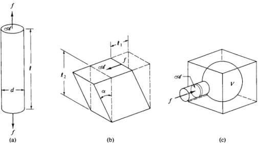
Another type of limiting behavior is that of an ideal elastic body. Such a body deforms or shows strain which is proportional to the applied unbalanced force or stress. The ratio of stress over strain is called the elastic modulus, and a crystal of cubic symmetry has three kinds of elastic modulus: Young's modulus Y (change in normal stress divided by the resulting relative change in length), shear or rigidity modulus G (change in tangential stress divided by change in the resulting
21-4 RHEOLOGY 9 0 7
/
(a) (b) (c)
FIG. 21-7. Diagrams explaining the definitions of the elastic constants, (a) Young9s modulus Y;
(b) shear modulus G; and (c) bulk modulus K. (st is area, dis diameter, I is length, Vis volume, and f is force.) [From J. R. Van Wazer, J. W. Lyons, Κ. Y. Kim, and R. E. Colwell, "Viscosity and Flow Measurement." Copyright 1963, Wiley (Interscience), New York. Used by permission of John Wiley & Sons, Inc.]
angle of extension), and bulk modulus Κ (change in hydrostatic pressure divided by resulting change in volume). These deformations are illustrated in Fig. 21-7.
A less isotropic solid has moduli that are different for different directions of stress—up to a maximum of 21 in all.
The subject of rheology is made considerably more complicated by nonideal behavior. A liquid whose viscosity decreases with increasing stress (such as increas
ing rate of flow or of stirring) is called pseudoplastic, if the viscosity increases with stress, the liquid is dilatant. These cases are illustrated in Fig. 21-8, in which rate of shear is plotted against the shearing stress. Referring to Eq. (2-57), / = η<$/ dv/dx,
the quantity dv/dx is the rate of shear, and f/<s/, the force differential per unit area, is the shearing stress.
FIG. 21-8. Shear versus stress plots. (1) Newtonian fluid; (2) pseudoplastic fluid; (3) dilatant fluid; (4) Bingham plastic; (5) pseudoplastic with a yield value; and (6) dilatant material with
a yield value.
6 4
5
0
S h e a r i n g stress
21-5 Liquid Crystals. Mesophases of Matter
There are a number of crystalline substances which show a very peculiar behav- ior on warming. For example, the compound 5-chloro-6-«-heptyloxy-2-naphthoic acid,
exists in ordinary crystalline form. On heating to 165.5°C, the crystals collapse to a turbid, viscous melt which adheres to the walls of the container. If this is spread on a flat plate, one may see steps or ridges; it is birefringent, showing colored areas under polarized light and having different optical properties parallel and perpendicular to the plate. Further heating of the compound produces a second change, at 176.5°C, to a fluid but turbid liquid. Only at 201 °C does final true melting to a clear liquid occur.
Cl
An ideal elastic solid shows no shear at any shearing stress, but actual solids will have a yield point beyond which flow begins to occur. A solid is known as a Bingham plastic if, once flow takes place, the rate of shear is proportional to the shearing stress in excess of the yield value, illustrated by curve 4 in the figure.
Curves 5 and 6 are those for pseudoplastic and dilatant materials showing a yield value.
The measured viscosity of a system is given by the ratio (f\stf)\(dv\dx). Thus Bingham and pseudoplastic solids as well as non-Newtonian liquids have viscosities that are dependent on the rate of shear.
The situation is yet worse than that described since the measured viscosity can vary with time as well as with shearing stress. A liquid which becomes more fluid with increasing time of flow is said to be thixotropic, while if the opposite is true, we say it exhibits rheopexy.
Examples of these types of behavior are as follows. Gases and pure single- phase liquids exhibit Newtonian viscosity, while suspensions, slurries, and emul- sions are apt to show dilatant behavior—a common example being that of a thick starch paste. It is often difficult to distinguish between behaviors 2 and 5 of Fig. 21-8, that is, between a pseudoplastic fluid and a pseudoplastic solid with yield value; the term pseudoplastic is therefore often applied without attempting to make the distinction. Materials in this general category include melts or solu- tions of high molecular weight solutes. Household paints are often pseudoplastic so as to brush easily, yet not run; the same is true for printing inks.
Ordinary crystalline solids will always have a yield value, but often a very high one. That for metals is around 10-50 kg m m- 2, for example—flow begins to occur once this yield pressure is exceeded.
Some gels are thixotropic—they will liquify on shaking. The same is true of certain types of suspensions, such as of bentonite clay. They settle very slowly on
standing, but rapidly if tapped gently.
21-6 POLYMERS 909
(a) (b)
F I G . 21-9. Molecular arrangements for (a) smectic mesophase, (b) nematic mesophase, and (c) isotropic liquid.
This type of behavior is called liquid crystalline because of the combination of properties exhibited, and the phases involved are called mesophases (lying between crystalline and liquid). Liquid crystals tend to occur with compounds that are highly asymmetric in shape, often having well-separated polar and nonpolar portions to the molecule. The two types of mesophases described here are called smectic and nematic, and the type of order present is illustrated in Fig. 21-9. In the smectic phase the molecules have retained their parallel orientation but have lost the crystalline regularity in the spacing between them so that successive layers no longer match. In the nematic phase the molecules, while still parallel, have further lost their planar array.
A great many biological structures might be called liquid crystalline—there is partial but not complete ordering between molecular units. Muscle fibers show double refraction; sperm cells may possess a truly liquid crystalline state; a solu- tion of tobacco mosaic virus contains nematic-type micellar units. At a simpler level, cholesterol and its derivatives may show both a smectic and a so-called cholesteric mesophase, the transition from the latter to isotropic melt occurring at around body temperature. The change from isotropic to cloudy liquid crystalline phase is very sensitive to electric fields and, in thin layers, to how the molecules orient in adsorbing at the boundary interfaces. Some phenomenal practical applica- tions have resulted; one example is in the display of time on watches.
21-6 Polymers
The great importance of polymers hardly needs to be stressed. Biological poly- mers such as proteins and nucleic acids are central to the functioning of living things. Natural polymers such as rubber and the host of synthetic ones such as polytetrafluoroethylene ("Teflon"), polyethylene, and polystyrene are vital mate- rials to our technology.
There are perhaps three major aspects to the general subject. The first is that of the chemistry of polymers—their synthesis and degradation reactions; the second important subject is the physical chemistry of polymer solutions; and the third is that of the overall configurational structure of polymers. The material that follows is intended merely to be illustrative of each of these very large fields.
A. Polymerization Chemistry and Kinetics
The characteristic feature of a polymer is that it is composed of a large number of identical or at least similar units which are chemically bonded together. The compound which forms the "repeating" unit is called the monomer. Thus in polystyrene,
—CH—CH
2—(CH—CH2)n—CH—CH2 —,
Φ Φ Φ
the monomer unit is styrene, C6H5C H = C H2. Polymers of this type are called linear polymers. Other examples include polyethylene, polyvinyl chloride, poly- acrylic esters and biological polymers such as proteins and polysaccharides. If more than two polymer forming functions are present, as with divinyl benzene ( C H2= C H — C6H4— C H = C H2) , then cross-linked chains form, yielding a three- dimensional network. Cross-linking may also be induced to occur in an already formed linear polymer. Thus in the case of rubber,
—CH
2—CH—CH—CH2—CH
2—C=CH—CH2 —,
CH
I I 3CH
3,
the natural linear polymer chains may be tied at random positions by mixing in sulfur and heating to form C—S—C bonds bridging two chains. Irradiation of polyethylene with gamma rays knocks off hydrogen atoms at random points and the resulting active carbon atoms can then bond to a neighboring chain.
Polymerization reactions generally occur by one of two types of mechanism.
Vinyl monomers are polymerized by a free radical process such as that for ethylene,
Ro*
~h C H 2 = C H 2 —*~Ro—CH
2—CH
2*
Ro—CH2—CH2* ~h C H 2=C H 2
—Ro—CH
2—CH2—CH2—CH2*
(21-12)where R0- is an initiating radical produced by some catalyst such as a peroxy acid,
Ο
II
RCOOH,
or photochemically. Styrene will polymerize just on heating in the presence of oxygen.
The formal kinetic scheme for the radical mechanism is as follows:
R0 + Μ i M r (initiation), (21-13) M r + Μ i Μ2·, Μ,· + Μ i Μ3· (propagation), (21-14)
Μη· + M r ^ Mn + Μβ (or Mn + 8) (termination). (21-15) Application of the stationary-state hypothesis (Section 14-4C) yields
R{ = Rt = kt J £ ( Μη· ) ]2 = kt(M-)2, (21-16) where Ri and Rt are the initiation and termination rates, respectively, it being
assumed that any two radical chains react to terminate with the same rate constant
21-6 POLYMERS 911 kt; ( M ) denotes the total radical concentration, £w ( Mw) . If we further assume that kx = k2 = kn = kv for the reactions of Eq. (21-14), where fcp is the common propagation rate constant, then the rate of disappearance of monomer is
=( Μ ) Α ΓΡΣ( Μ . · ) . ( 2 1 - 1 7 )
η
On substitution for (Μ·) from Eq. (21-16), we obtain
- f = M | ) '
S» « » - « )
In general each polymerization system must be subjected to separate kinetic analysis since the appropriate set of approximations may vary. A particularly simple special case of Eq. (21-18), however, is that in which Rt is photochemical and therefore given by φΙ& , where φ is the quantum yield for radical production and 7a is the number of quanta of light absorbed per unit volume and time. A point implicit in schemes such as this is that after some time t there will be a distribution of polymer molecular weights. A more detailed analysis would predict both the average molecular weight and the breadth of the distribution.
A second type of mechanism is that in which a Lewis acid such as A1C13 or an ordinary strong protonic acid such as H2S 04 adds a proton to the monomer. A typical sequence is that for the production of butyl rubber by the polymerization of isobutylene,
CH3 CH3 CH3 CH3 CH3 CH3
— I I I I I I
H+ C H2= C ^ C H2= C ^ C H2= C - > C H3- C - C H2- C - C H2- C - . (21-19) I I I I I I
CH3 CH3 CH3 CH3 CH3 CH3
More recently, transition metal ions have been found to be excellent catalysts for polymerization reactions, often giving highly stereoregular or isotactic polymers.
(A polymer such as polystyrene is isotactic if, when the chain is stretched out, all of the phenyl groups are on one side.)
A related mechanism is that whereby water is eliminated between two functional groups. Thus a protein chain,
R Ο R Ο R Ο I II I II I II- H - C - N - C - ( C - N - C - )n- C - N - C - H ,
I I I I I I Η Η Η Η Η Η
forms on elimination of water between R C O O H and R N H2 groups. The R's vary down the chain in natural proteins but may be the same in synthetic polypeptides.
As another illustration, nylon results from the condensation of adipic acid ( H O O C ( C H2)4- C O O H ) with hexamethylenediamine ( H2N ( C H2)6N H2) . These various polymerizations follow kinetic schemes similar to that of Eqs. (21-13)- (21-15).
B. Polymer Solutions
The study of polymer solutions can be regarded as a branch of colloid chemistry.
As with colloidal suspensions, one is interested in the distribution of particle sizes (in this case, polymer molecular weights), in the shape of the particles, in their
interaction with the solvent medium, and in the general physical properties of the system.
1. MOLECULAR WEIGHT. The general methods for molecular weight determina
tion are discussed in Section 10-7. For polymers these include measurement of osmotic pressure, diffusion rate, sedimentation equilibrium and sedimentation rate, and light scattering. If a range of molecular weights is present, a given method will yield either a number-average or a weight-average molecular weight; if both types of average molecular weight can be determined, their ratio provides a measure of the broadness of the molecular weight distribution.
2. VISCOSITY. There is an additional method of molecular weight estimation which makes use of viscosity measurements. Einstein showed in 1906 that for a dilute suspension of spheres in a viscous medium
lim ( η , η ο] ~ 1 = 2.5, (21-20)
φ->0 φ
where η and η0 are the viscosities of the solution or suspension and pure solvent, respectively, and φ is the volume fraction of the solution occupied by the spheres.
The fraction η/η0 is called the viscosity ratio or relative viscosity ψ , and
Kvho)
— 1] is called the specific viscosity η8Ρ. In the case of a polymer solution the concentration C is usually given as grams per cubic centimeter and ^p/lOO C is called the reduced viscosity and its limiting value as C approaches zero is the intrinsic viscosity [^].+ Since φ = v2C, where v2 is the specific volume (strictly,the partial specific volume) of the polymer in cubic centimeters per gram, it follows from Eq. (21-20) that [η] = 0.025t>2. The specific volume as determined from [η]
will in general be larger than that obtained from the density of the dry polymer, the difference being attributed to bound solvent.
The factor 2.5 in Eq. (21-20) applies to the case of spheres, and linear polymers are, of course, not spherical, in the sense of the molecule being a long chain. On the other hand, the completely extended configuration is a very improbable one, and the situation is more like that illustrated in Fig. 21-10, which shows various random coils. The problem is essentially the statistical one of calculating the most probable end-to-end distance d assuming the polymer to consist of n flexible links;
d, as might be expected, turns out to be proportional to the square root of the chain length. The proportionality constant depends, however, on the balance between solvent-chain and chain-chain interactions. In a "good" solvent, the random coil will be very extended, while in a " p o o r " solvent, the chain prefers its own environment and therefore assumes a compact configuration. While none of these configurations is exactly spherical, Eq. (21-20) can still be used, but with an empirical parameter ν in place of the Einstein coefficient 2.5, and ν evidently will depend on the nature of the solvent as well as on that of the polymer.
An alternative development of Eq. (21-20) is the following. If φ0 denotes the volume fraction calculated using v2 for the dry polymer, then the correct φ is given by φ0β, where β is the ratio of the hydrated to dry specific volumes. The dry
+ The definitions a b o v e are the traditional ones. The current r e c o m m e n d a t i o n is that η/η0 be called the viscosity ratio and n o t relative viscosity; that [(ηΙη0) — 1 ] / C be called the viscosity number; and that the limiting value as C approaches zero, or limiting viscosity number, be designated [η].
21-6 POLYMERS 913
F I G . 21-10. Random coils of the same length and same general configuration but of increasing tightness or in successively poorer solvents.
volume of a polymer is, of course, proportional to its molecular weight M. The hydrated volume will be proportional to d3, or to M3/2, so β should be proportional to Μm. Thus Eq. (21-20) can be put in the form
[η] = KM1/2. (21-21)
If, however, the polymer were a rigid rod of length d, its effective volume would be that swept out by the tumbling of the rod. The "hydrated" volume is now propor
tional to M3, and β is proportional to M2.
The exponent in Eq. (21-21) can thus be expected to vary depending on the stiffness of the polymer, and in an equation proposed by M. Staudinger in 1932 it is treated as an empirical parameter:
[η] = KMa. (21-22)
The experimental observation is that Κ and a are approximately constant for a given type of polymer and a given solvent. Polymers of about the same chemical composition may differ greatly in molecular weight and Eq. (21-22) allows the relative molecular weights of different preparations to be determined. If two preparations of different known molecular weight can be obtained, then Κ and a can be evaluated, and absolute molecular weights may then be found for any other sample. It might be mentioned that if a range of molecular weights is present in the
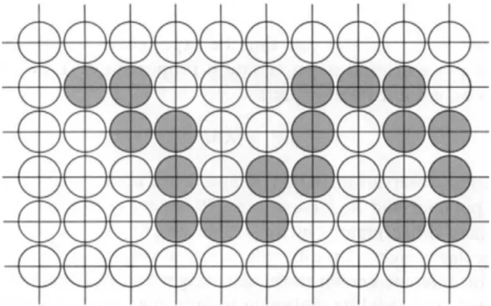
F I G . 21-11. Illustration of the statistical fitting of solvent molecules (open circles) and monomer units (shaded circles) on a two-dimensional lattice.
sample, then the value calculated by means of Eq. (21-22) will be an average lying between the number- and weight-average values.
This type of study has been made for a number of types of polymer and values of a are usually in the range 0.5-1.1. As expected, a decreases if one goes from a good to a poor solvent. That is, the relatively compact configuration present in a poor solvent behaves more like a sphere than a rod.
3. THERMODYNAMICS. One approach to the statistical treatment of polymer solu
tions is to consider the solution as consisting of a number of cells or sites. Each site may be occupied by a solvent molecule or by one link or monomer unit of the polymer; as illustrated in Fig. 21-11, the requirement is that successive links occupy adjacent sites. One then treats the "solution" of links as a regular one (Section 9-CN-2) or essentially according to the model of Section 9-2E, but with the added aspect that the entropy of the links is reduced because of their having to remain connected.
The vapor pressure or activity of the polymer is then given by an equation similar to Eq. (9-17) and varies with solution composition in a way similar to that shown in Fig. 9-9. Thus for a > 2, there is a maximum and a minimum, corre
sponding to partial miscibility; however, the effect of the entropy complication is to distort the behavior in the direction of making intermediate compositions less probable than for an ordinary regular solution. As a consequence, one finds that for oc > 2, the dilute solution tends to be very dilute and the concentrated solution very concentrated, corresponding to slightly solvated polymer in equilibrium with a dilute solution. This explains the experimental observation that polymers tend to be either slightly soluble or quite soluble in a given solvent.
The quantity α in Eq. (9-17) is actually an interaction energy ω divided by kT.
The critical condition is therefore that α = ω/kTc = 2, or Te = ω/lk. This rela
tionship accounts for the common observation that below a critical temperature a polymer will not be very soluble, whereas above this temperature it is almost completely miscible with the solvent.
4. SECONDARY STRUCTURE. The primary structure of a polymer is that of the chemically bonded chain itself, including its stereochemistry. Since we are dealing with a macromolecule, there is a second level of structure, namely that of the polymer chain as a whole. We saw in the preceding section that linear polymers
21-6 POLYMERS 915
in solution assume a random coil configuration, for example. The coil becomes tighter the poorer the solvent or the more strongly interacting the polymer chain is with itself.
As a limiting case of this last situation, amino acid polymers, that is, proteins, can form hydrogen bonds between various portions of the chain. L. Pauling proposed a now widely accepted structure known as the α-helix. The helix makes one turn for every 3.7 amino acid residues, thus allowing hydrogen bonding between the CO and N H groups of adjacent coils.
In the case of the nucleic acids, the primary structure is that of a linear polymer in which adenine (A), guanine (G), cytosine (C), and thymine (T) rings are linked by phosphate groups; adjacent chains are hydrogen bonded as shown in
(a) (b) F I G . 21-12. Structure of DNA. (a) Hydrogen bonding between adenine (A) and thymine (T)
and between cytosine (C) and guanine (G). (b) Two strands held in a double helix by C - G and T - A hydrogen bonds. [See Μ. H. F. Wilkins and S. Arnott, J. Molec. Biol. 1 1 ,3 9 1 (1965).] [Part (b)from A. White, P. Handler, and E. L. Smith, "Principles of Biochemistry," 4th ed. Copyright
© 1968, McGraw-Hill, New York. Used with permission of McGraw-Hill Book Company.]
Fig. 21-12. The secondary structure is that of a double helix in which C - G and A - T pairs form hydrogen bonds. The detailed configuration of these hydrogen bonds is at present subject to some controversy.
The ordinary denaturation of proteins and nucleic acids generally consists of a loss of the secondary structure but not of the primary structure. Intermediate situations are possible, too, in which part of the polymer has the helical configura
tion and part that of random coils. It has been possible in some cases to observe helix-coil transitions.
Finally, one may speak of a tertiary structure. A protein helix is still a long unit and one which may fold in on itself. Regions which have few polar groups find water a poor solvent, and hence tend to approach each other—the effect has been rather misnamed as hydrophobic bonding. The consequence is that native proteins tend to form a tertiary structure which is more or less globular and with the nonpolar groups in the interior.
Several very interesting phenomena may occur if there is relative motion between a charged surface and an electrolyte solution; these are called electrokinetic effects.
The surface is ordinarily either that of a solid particle suspended in the solution or the solid wall of tube down which the solution flows. What happens is essentially that a charged surface experiences a force in an electric field or, conversely, that a field is induced by the motion of such a surface relative to the solution. Thus if a field is applied to a suspension of colloidal particles, these will move or, alternative
ly, if a solution is made to flow down a tube an electric field develops. In each case there is a plane of shear between the surface and the solution, a plane which lies within the electrical double layer. The potential at this plane will not be φ0, but some lower value called the zeta potential ζ. The zeta potential does give a measure of φ0 , however, and one important application of electrokinetic phenom
ena is to the measurement of ζ and hence estimation of φ0 .
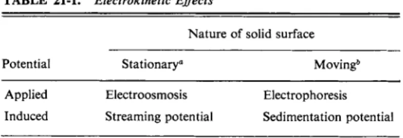
There are four types of electrokinetic effect, depending on whether the solid surface is stationary (as a wall) or moves (as a particle) and whether the field is
SPECIAL TOPICS 21-ST-l Electrokinetic Effects
T A B L E 2 1 - 1 . Electrokinetic Effects
Nature of solid surface
Potential Stationary0 Moving*
Applied Electroosmosis Electrophoresis Sedimentation potential Induced Streaming potential
a For example, a wall or apparatus surface.
b For example, a colloidal particle.
SPECIAL TOPICS, SECTION 1 917 applied or induced. In electrophoresis an applied field causes suspended particles to move, while in the sedimentation potential effect the motion of the particles in a centrifugal field induces a field. If the solid surface is that of the wall of a tube, application of a potential gradient or field induces a flow of solution, or electroosmosis, while a forced flow of solution induces a potential gradient or streaming potential. The four effects are summarized in Table 21-1. We will consider only two of them, however, namely electrophoresis and the streaming potential effect.
A. Electrophoresis
The most familiar type of electrokinetic experiment consists of setting up a potential gradient in a solution containing charged particles and determining their rate of motion. If the particles consist of ordinary small ions, the phenomenon is one of ionic conductance, treated in Chapter 12. As shown in Section 12-5, the velocity of an ion in a field F is
vt = ζ,βω,Έ [Eq. (12-27)],
where ω{ is the mobility and t\ will be in centimeters per second if e is in esu and F in esu volts per centimeter. Alternatively, by Eq. (12-28), vt = wtF, where ut is the electrochemical mobility and F is now given in ordinary volts per centimeter;
also, by Eq. (12-31), λ, = wfF.
In the case of a macromolecule, the total charge zt is not known, and it is customary to refer to the motion of such molecules in an electric field as electro- phoresis.
However, if the molecular weight is known, then the radius can be calculated assuming the shape to be spherical. This allows estimation of the friction factor f from Stokes' law, Eq. (10-33), and hence of ω = \\f. Alternatively, if the diffu
sion coefficient can be measured, then f can be obtained without any geometric assumptions from Eq. (10-41). The charge on the polymer molecule may then be calculated from the electrophoretic velocity using Eq. (12-27).
As would be expected from the discussion of the acid-base equilibria of amino acids (Section 12-CN-3), the net charge on a protein is very /?H-dependent. For each protein there will be some one pH at which ζ and hence the electrophoretic velocity is zero. Conversely, at a given pH each protein will have a characteristic velocity in an electric field, depending both on its molecular weight and on its net charge. A mixture of proteins will therefore separate into different velocity groups in an electrophoresis experiment. See Section 12-5D, and especially Fig. 12-5.
We turn now to colloidal particles. As with macromolecules, the charge is not known; in addition, the size cannot be determined very accurately, although it may be possible to estimate particle radii from microscopic (optical or electron) examination. Ordinary molecular weight determination is, of course, not possible (why ?) nor is the diffusion rate fast enough for a determination of / . As noted in the introduction to this section, we assume instead that the particle is large enough for its interface with the solution to be treated as planar, and apply electrical double layer theory.
The complication mentioned at the beginning of this section is that, as illustrated in Fig. 21-13, there is undoubtedly a layer of solvent molecules and electrolyte ions which is strongly enough held that it moves with the particle rather than
with the solution. We must deal, therefore, with the plane of shear rather than with the actual interface; the potential ψ0 is reduced to some value φ = ζ at this plane, called the zeta potential, and σ0, to some value as. The remainder of the diffuse double layer must still balance as, or, by Eq. (21-9), as = $™=s ρ dx. The
"center of gravity" of this portion of the double layer is taken to be at the point where φ has dropped to l/e of ζ, at distance τ from the plane of shear.
As a first approximation, the situation is likened to that of a parallel plate condenser, for which the standard formula gives Δ V — 4nqd/D<srf, where J Κ is the potential difference across the plates, d is their separation, is their area, and D is the dielectric constant. One plate carries charge +q and the other carries —q.
We now equate Δ V to ζ, d to r, and q/st to os to obtain
σ . = . (21-23) We next proceed to balance the electrical force acting per square centimeter of
the particle with that due to viscous drag. The first is just osF , where F is the field, and the second may be obtained from the defining equation for viscosity, Eq. (2-57).
We assume that the relative velocity between the particle and the solution drops linearly with distance from ν at χ = s to 0 at χ = τ and therefore write dv/dx = ν/τ, which gives the viscous force or drag per square centimeter as ην/τ. On equating the two forces, we obtain
— = Ι γ - » ϊ '
<2 1-2 4>where in the second form, F is expressed in volts per centimeter. An alternative form results on combination with Eq. (21-23):
ν = ψ*-. (21-25) Λπη
F I G . 21-13. The diffuse double layer, showing the plane of shear at which φ has the value £, the zeta potential.
SPECIAL TOPICS, SECTION 1 919
All of the fundamental statements have been written in the esu system insofar as electrical quantities are involved, but one usually reports ζ in volts (actually, millivolts), having measured F in volts per centimeter. If one converts ζ to milli
volts by means of the factor 1000/300 and F to volts per centimeter by the factor 1/300, one obtains a more practical form of Eq. (21-25):
ζ= 12.9 (21-26) where, in addition, ν is in microns per second and D and η have been taken to be
for water at 25°C. Thus if a colloidal particle moves 50 μ s e c- 1 in a field of 10 V c m- 1, its zeta potential is 65 mV, positive or negative depending on the direction of motion relative to the field. The field may be applied by means of nongassing electrodes at each end of a tube containing the colloidal suspension and the rate of motion of individual particles observed under a microscope; the instrument is called a zetameter.
Most measured zeta potentials are in the range of ± 1 0 0 mV for lyophobic colloids, but with actual values dependent on the nature and concentration of the electrolyte. Table 21-2 gives some data on a gold sol which show that the charge decreases and then reverses with increasing A l3 + ion concentration. Note that the sol is stable if the particles are charged but flocculates rapidly if the zeta potential is small.
β. Streaming Potential
If an electrolyte solution flows through a tube, one observes a potential differ
ence between the inflowing and outflowing solution. The physical basis for the effect is that the flowing solution carries with it the charge density as in the diffuse double layer, so that there is in effect an electrical current at the wall. The current is just / = 2nrasvT, where vT is the streamline velocity at distance τ from the wall; it is thus proportional to the surface area and, by Eq. (21-23), to the zeta potential. A potential drop Ε develops in the electrolyte solution until a counter current i = E/R, develops, where R is the resistance of the solution, such as to just balance the wall current. It is this steady-state potential that is called the streaming potential.
The actual derivation is somewhat in the same vein as that of the Poiseuille equation given in Section 8-10. Assuming streamline flow, the velocity at a
T A B L E 2 1 - 2 . Flocculation of Gold Sol
Concentration
of Al3+ Electrophoretic velocity
(equiv l i t e r- 1 χ 10e) (cm V -1 s e c -1 χ 106) Stability 0 3.30 (toward anode) Indefinitely stable
21 1.71 Flocculates in 4 hr
— 0 Flocculates spontaneously
42 0.17 (toward cathode) Flocculates in 4 hr
70 1.35 Incompletely flocculated after 4 days
radius χ from the center of the tube is
P(r2 _ χ2)
V = 4 ψ ^ [ E q- ( 8"6 4 ) ]'
where Ρ is the pressure drop and r the radius of the tube, which is of length /.
The double layer is centered at χ = r — r , and substitution into Eq. (8-64) gives
v* = ^ (21-27) if the term in r2 is neglected. The current due to the motion of the double layer
is then
ι = 2nrasva (21-28)
or
i = ^ ^ . (21-29) Ψ
If κ is the specific conductivity of the solution, then the actual conductivity of the liquid in the tube is C = πΓ2κ/1 and, by Ohm's law, the streaming potential is just Ε = i/C. Combining these equations, we have
τ σ0Ρ
Ε = —ζ- (21-30)
or, using Eq. (21-23),
E = - ^ - . (21-31)
Αστη w v /
4πηκ A practical form of Eq. (21-31) is
Ε - 8.0 χ l O "5^ , (21-32)
where ζ is now in millivolts and Ρ in atmospheres; C is the electrolyte concentra
tion in equivalents per liter and Λ is the equivalent conductivity. Water at 25°C is assumed. Thus for a pressure drop of 10 atm, a zeta potential of 50 mV, and ΙΟ"5 Ν aqueous NaCl at 25°C (equivalent conductivity 126), Ε = 32 V. As this example illustrates, the electrolyte must be quite dilute if an appreciable effect is to occur.
Streaming potentials may cause trouble in the filtering of dilute electrolyte solutions, especially nonaqueous ones whose electrolyte concentration and hence specific conductivity may be quite small. A quite real hazard developed in the early days of jet aircraft—the high pumping rate of the kerosene fuel led to streaming potentials large enough to cause sparks. The problem has since been eliminated by incorporating small amounts of conducting solutes in the fuel.
G E N E R A L R E F E R E N C E S
ADAMSON, A . W. ( 1 9 7 6 ) . "The Physical Chemistry of Surfaces," 3rd ed. Wiley (Interscience), N e w York.
BILLMEYER, F. W., J R . ( 1 9 6 2 ) . "Textbook of Polymer Science." Wiley (Interscience), N e w York.
G R A Y , G. W. ( 1 9 6 2 ) . "Molecular Structure and the Properties o f Liquid Crystals." Academic Press, N e w York.
EXERCISES 921 K R U Y T , Η . R . (1952). "Colloid Science." Elsevier, N e w York.
M C B A I N , J. W . (1950). "Colloid Science." Heath, Indianapolis, Indiana.
MYSELS, K . J . (1959). "Introduction t o Colloid Chemistry." Wiley (Interscience), N e w Y o r k . V A N W A Z E R , J . R . , L Y O N S , J . W . , K I M , Κ . Y . , A N D C O L W E L L , R . E. (1963). "Viscosity a n d F l o w
Measurement." Wiley (Interscience), N e w York.
VERWEY, E . J . W . , A N D OVERBEEK, J . T H . G . (1948). "Theory o f the Stability o f Lyophobic Colloids." Elsevier, N e w York.
W H I T E , Α., H A N D L E R , P., A N D SMITH, E. L. (1968). "Principles o f Biochemistry," 4th ed. McGraw- Hill, N e w York.
C I T E D R E F E R E N C E
A D A M S O N , A . W . (1976). "The Physical Chemistry o f Surfaces," 3rd e d . Wiley (Interscience), N e w York.
EXERCISES
T a k e as exact numbers given t o o n e significant figure.
21-1 Calculate the attractive potential due t o dispersion forces between two platelets (say, o f a colloidal suspension o f a mica, vermiculite) for which Η = 3.0 χ 1 0 ~1 8 erg and the surface- to-surface distance is 250 A. Express your result in units o f kT (at 25°C).
Ans. 3.1 χ 1 01 0c m -2.
21-2 For what value o f φ is εφ/kT = 1 at 25°C?
Ans. 25.7 m V .
21-3 A surface o f potential 51.4 m V is in contact with a 0.1 Μ solution o f N a C l at 2 5 ° C . Cal
culate the concentrations o f N a+ and o f Cl~ ions at the surface.
Ans. ( N a+) = 0.0135 M, (CI") = 0.739 M.
21-4 Referring t o Exercise 21-3, calculate φ a n d ( N a+) , (CI"), a n d t h e charge density ρ at a distance o f 15 A from the surface.
Ans. 10.8 m V , 0.0656 M , 0.152 M , 0.0867 m o l e o f charge l i t e r "1 o r 2.51 x 1 01 0 esu c m "8.
21-5 Still referring t o Exercise 21-3 (and 21-4), calculate the repulsion energy per square centi
meter between t w o charged surfaces for φ0 = 51.4 m V w h e n in 0.1 Μ N a C l a n d 15 A apart (at 25°C).
Ans. 0.144 erg c m- 2.
21-6 Calculate the attractive potential between t w o slabs o f area 1 0- 9 c m2 each when separated by 15 A. U s i n g the result o f Exercise 21-5, obtain the net interaction energy for these slabs (or colloidal platelets) when immersed in 0.1 Μ N a C l at 25°C. Assume Η to b e 3.0 χ 1 0- 1 3 erg.
Ans. Attractive potential energy is 3.54 χ 1 0 ~1 0 erg;
net potential energy i s —2.10 χ 1 0 "1 0 erg (attractive).
21-7 A
Theological
study o f a certain fluid gives y = 0.1 χ + 2x2, where y is the rate o f shearin s e c o n d- 1 and χ is the shear stress in dynes per square centimeter. Calculate the viscosity at a shear stress of 10 dyn c m- 2. What type of rheological behavior is being exhibited?
Ans. 0.0498 P.
21-8 Suppose that the polymerization kinetics of Eqs. (21-14) and (21-15) is followed, but that the initiation step is photochemical, with radicals produced by the process R ^> 2 M . S h o w that Eq. (21-18) b e c o m e s —d(M)/dt = £P(2<£//A:t)1 / 2(M), where φ is the quantum yield and / the rate of absorption of light quanta.
21-9 The relative viscosity of a solution of polystyrene has the following values:
C'(g per 100 c m3) 0.08 0.12 0.16 0.20
ητ 1.213 1.330 1.452 1.582
Find [η] and estimate v2 for the polymer. Calculate Κ of Eq. (21-21) if the molecular weight of the polymer is 250,000 g m o l e- 1, and calculate the relative viscosity of a 0.10 g per 100 c m8 of solution of polymer of molecular weight 500,000. (The slope of the plot of ijep/lOOC should vary as [η]2.)
Ans. [η] = 2.49, v2 = 100 c m8 g "1, Κ = 4.98 x 1 0 "8, ητ = 1.395.
P R O B L E M S
21-1 Derive Eq. (21-2) from Eq. (21-1) by carrying out the required triple integration.
21-2 Calculate the interaction energy in calories per mole for an argon atom adsorbed on a hypothetical argon surface; assume the atom-surface distance to be 3.5 A. ( N o t e Table 8-8.)
21-3 The value of χ for which ψ/ψ0 is 1/e is called the double layer "thickness" τ. Calculate τ as a function of concentration of N a C l at 25°C up to 0.5 Μ and plot the result.
21-4 S h o w that Eq. (21-9) can be phrased as σ =
—(DI4n)Wldx)
x = 0 and further s h o w that an approximate value for σ isϋκψ
0/4π.
21-5* Calculate, using Eqs. (21-3) and (21-10), the net interaction energy in units o f kT for t w o colloidal platelets as a function of their distance of separation and for κ = 1 05 c m " \ 1 06 c m "1, and 1 07 c m "1. A s s u m e that Η = 3 χ 1 0 "1 8 erg, ψ0 = 25.6 m V , Τ = 25°C, and assume an a q u e o u s N a C l m e d i u m . F o r each κ value, plot your results as e/kT versus χ in angstroms up to about 2 0 0 A. T h e area of each platelet is 1 0 "9 c m2.
21-6 The following data were obtained for the viscosity of nitrocellulose in butyl acetate:
C ( g per 100 c m8) 0.032 0.075 0.135 0.180
ηΤ 1.540 2.323 3.964 8.025
Calculate the intrinsic viscosity of this polymer and its specific volume.
21-7 The following relative viscosities were measured for a polyisobutylene in cyclohexane.
C ( g per 100 c m8) 0.050 0.152 0.271 0.441
ητ 1.2895 2.067 3.312 6.579
Calculate the molecular weight of the polymer if the constants in Eq. (21-22) are a = 0.73 and Κ = 5.1 χ Ι Ο- 4.
21-8 The viscosity of a globular protein is investigated at 5°C using an Ubbelohde viscometer (based o n the Poiseuille equation, Section 8-10; note that Px — P% is proportional to