Algal cell response to laboratory-induced cadmium stress: a multimethod approach
Nadica Ivošević DeNardis*1, Jadranka Pečar Ilić1, Ivica Ružić1, Nives Novosel2, Tea Mišić Radić1, Andreas Weber3, Damir Kasum1, Zuzana Pavlinska4,5, Ria Katalin Balogh6, Bálint Hajdu6, Alzbeta Marček Chorvatova4,5, Béla Gyurcsik6
1Division for Marine and Environmental Research, Ruđer Bošković Institute, POB 180, 10000 Zagreb, Croatia,2Department of biology, Faculty of Science, University of Zagreb, Rooseveltov trg 6, 10000 Zagreb, Croatia, 3Department of Nanobiotechnology, Institute for Biophysics, University of Natural Resources and Life Sciences, Muthgasse 11, 1190 Vienna, Austria, 4Department of Biophysics, Faculty of Natural Sciences, University of Ss. Cyril and Methodius, nam. J Herdu 1, 91702 Trnava, Slovakia, 5Department of Biophotonics, International Laser Centre, Ilkovicova 3, 84104 Bratislava, Slovakia, 6Department of Inorganic and Analytical Chemistry, University of Szeged, Dóm tér 7, H-6720 Szeged, Hungary
*Corresponding author:
Tel: +385 1 4561-128 Fax: +385 1 4680-242
E-mail address: ivosevic@irb.hr (N. Ivošević DeNardis)
Abstract
We examined the response of algal cells to laboratory-induced cadmium stress in terms of physiological activity, autonomous features (motility and fluorescence), adhesion dynamics, nanomechanical properties and protein expression by employing a multimethod approach. We develop a methodology based on the generalized mathematical model to predict free cadmium concentrations in culture. We used algal cells of Dunaliella tertiolecta, which are widespread in marine and freshwater systems, as a model organism. Cell adaptation to cadmium stress is manifested through cell shape deterioration, slower motility and an increase of physiological activity. No significant change in growth dynamics showed how cells adapt to stress by increasing active surface area against toxic cadmium in the culture. It was accompanied by an increase in green fluorescence (most likely associated with cadmium vesicular transport and/or beta carotene production), while no change was observed in the red endogenous fluorescence (associated with chlorophyll). To maintain the same rate of chlorophyll emission, the cell adaptation response was manifested through increased expression of the identified chlorophyll-binding protein(s) that are important for photosynthesis.
Since production of these proteins represents cell defence mechanisms, they may also signal the presence of toxic metal in seawater. Protein expression affects the cell surface properties and therefore the dynamics of the adhesion process. Cells behave stiffer under stress with cadmium and thus the initial attachment and deformation are slower. Physicochemical and structural characterizations of algal cell surfaces are of key importance to interpret, rationalize and predict the behaviour and fate of the cell under stress in vivo.
Keywords: adhesion kinetics, autofluorescence, cadmium bioavailability, cell stress adaptation, nanomechanics, protein expression
Introduction
Microalgae play a fundamental role in aquatic ecosystems and have developed various strategies to cope with the presence of elevated environmental metal levels (Wang and Wang 2009). Microalgae are frequently used to evaluate the toxicity of heavy metals in the environment for remediation needs (Folgar et al. 2008; Imani et al. 2011; Shafik 2008) or to signal pollutants (Guihéneuf et al. 2016).
Cadmium is a non-essential trace metal recognized as a major pollutant of the marine environment, constituting a hazard to marine organisms. It is well known that the response of green algal cells under heavy metal stress includes the allocation of carbon flux to the synthesis of osmolytes and putative antioxidant molecules (e.g. sugars and β-carotene) (Einali et al. 2017). The amount of chlorophyll also varies under such conditions (Nikookar et al. 2005; Saha et al. 2018). An excess of transition metal ions in the environment may also significantly alter the ultrastructure, increase or decrease growth, chlorophyll content, protein and the antioxidant activities within cells (Sacan et al.
2007; Taha et al. 2012; Visviki and Rachlin 1994; Wikfors et al. 1991). Some of the expressed proteins may be related to temporary storage and the carrier function of chlorophyll and its late precursors, as well as to its antioxidant and photoprotective functions (Belghith et al. 2015; Damaraju et al. 2011).
The mechanism by which algae tolerates cadmium has been studied extensively (Belghith et al. 2015;
Fisher et al. 1984;Folgar et al. 2008; García-Ríos et al. 2007; Shariati and Yahyaabadi 2006; Tsuji et al. 2002; Tsuji et al. 2003; Visviki and Rachlin 1994; Wikfors et al. 1991). Despite this, to the best of our knowledge data on the bioavailability of cadmium in solutions is limited in the literature. Free cadmium in solutions is harmful to living cells in culture. Metals bind to cell surface ligands, enabling transport inside cells, or attach to the membrane (Campbell et al. 2002). Fisher at al. (1984) reported that marine phytoplankton cells develop different strategies to accommodate toxic metals, such as metal exclusion (having a less metal-reactive surface), internal sequestering of the metal in harmless forms, an extracellular detoxification mechanism (binding cadmium to metallothionein-like proteins) (Tsuji et al. 2002), dumping the polypeptide-metal complex (Wikfors et al. 1991) and metal ion
incorporation into non-essential intracellular sites away from vital metabolic locations (Zmiri and Ginzburg 1983).
The aim of the current study was to examine the algal cell response to laboratory-induced cadmium stress in terms of physiological activity, autonomous features (motility, fluorescence), adhesion dynamics, nanomechanical properties and protein expression by employing a multimethod approach.
We developed a methodology based on the generalized mathematical model that predicts the free cadmium concentration in culture. Algal cells of Dunaliella tertiolecta are widespread in marine and fresh water systems, so we used this species as a model organism. Dunaliella is a single-celled, motile green algae that is relatively simple to cultivate as algal cells do not clump, do not aggregate and do not form chains. Dunaliella tertiolecta cells have no solid cellular cell wall in contrast to other green algae, which makes them susceptible to changes in the ecosystem and is why they are often used as a model organism in stress research. Physicochemical and structural characterizations of single algal cell surfaces are of key importance to interpret, rationalize and predict the behaviour and fate of the cell under stress in vivo.
Theory
Model for 1:1 complex formation of a single ligand with several metals
The process of metals complexation, which involves a 1:1 complex formation between a single ligand and each individual metal, can be described with following reaction scheme:
(1) where L is a single ligand, Mi denotes a particular trace metal among n possible different metal ions, and LMi denotes complexes formed between a ligand and each particular trace metal. The corresponding formation constant (i.e. equilibrium constant for the reaction between the metal ion and the ligand) of the complex Ki reads:
(2) L+ Mi LM ,i i1, 2, 3, n
(LM )
K , 1, 2,3,
(L)(M )
i i
i
i n
where (L), (Mi) and (LMi) represent concentrations of free ligand, particular free trace metal and their corresponding complex, respectively.
Here, we present a generalized mathematical model for the 1:1 complex formation of a single ligand with many trace metals, arranged according to the strength of complexation (i = 1, 2, 3, ... n). First, mass balance relations should be established:
(3) where LT denotes the total concentration of a ligand and MTi represents the total concentration of the particular trace metal, i.e. free (Mi) and bound (LMi). Further, by combining Eqs. (2) and (3) we can derive an equation for the free trace metal concentration:
(4) Finally, to determine the free ligand concentration using Eqs. (3) and (4) the following expression can be derived:
(5)
were MT represents the total trace metals concentration:
(6) and K is a special function of the free ligand concentration:
(7)
where
Ki* (i = 1, 2, 3, … n) represents different combinations of individual formation constants of the complexes (e.g. expression of K1* represents the mean of the inverse values of individual formation constants of the complexes, while the other Ki*s have more complicated expressions depending on the number i of trace metals involved)
and
1 1 1
L (L) (LM ) M (M )
n n n
T i T i i
i i i
(M )i M / 1 K (L) ,T i i i1, 2,3, n
1
L (L) / (L) M / (L) 1/ K M / (L) 1/ K
n
T T i i T
i
1
M M
n
T T i
i
1 2 * *
2
1
1 * 2
1
1
(L) (L) / K K / K
K
(L) / K (L) / K K 1/ K
n
n n
n i
i n
n n
i j i
i
(i = 1, 2, 3, … n; j = 1, 2, 3, … n) represents the mean product of individual pairs of formation constants of the complexes.
The simplest case of a single 1:1 complex formation of one ligand with one trace metal was previously defined by the commonly known “van den Berg-Ružić plot” showing the ratio of free and bound metals (van den Berg 1982; Ružić 1982). In a similar way, the ratio of free and bound ligands can also be obtained from Eqs. (2)–(3) and (5)–(6) of the generalized model for this simple condition:
(8) In the simple case of two 1:1 complex formations of a ligand with two trace metals the equation for the free ligand concentration (L) can be derived from the generalized model for the corresponding condition:
(9) where LT is the total concentration of the ligand (Eq. (10)), MT is the sum of the total concentrations MT1 and MT2 of two metals (Eg. (11)), K1 and K2 are formation constants of the complexes (Eq. (12)) while K1* and K2* represent two different combinations of individual formation constants of the complexes (Eq. (13)):
(10) (11) (12) (13) Further, based on the equations of the generalized mathematical model, we propose a new methodology for calculating concentration ranges of the free metal ion that is introduced as a main stressor in algal cells’ growth medium.
The following input data are needed for the model: total concentration of the ligand LT, total concentration of the particular trace metal MTi and corresponding formation constants of the complexes between a single ligand and each particular trace metal Ki.
K Ki j
(L) / LT (L) 1/ K MT (L) / MT
* 2 2*
(L) / LT (L) (L)(L) / K1 1/ K K1 / (L) 1/ K / MT
LT (L) (L M ) (L M ) 1 2
MT1(M ) (L M ), M1 1 T2 (M ) (L M )2 2
K1 (L M ) / (M )(L) ,1 1 K2 (L M ) / (M )(L)2 2
* *
2 2
K1 MT M / KT1 1M / K ,T 2 K2 MT M / KT1 2M / KT 1
Values of LT and MTi can be obtained using the Primary Trace Metal Stock Composition of Guillard’s (F/2) Marine Enrichment medium (Guillard 1975), which is widely used for experiments where algal cells grow in medium under ambient conditions.
Formation constants of the complexes Ki can be obtained from the NIST Standard Reference Database (Martell et al. 1998, 2004).
Reaction kinetics model for cell adhesion and spreading at the charged interface
The kinetics of organic particle adhesion to a charged interface can be described as a process involving three steps that were previously reported in detail (Ivošević DeNardis et al. 2012, 2015;
Ružić et al. 2010). Briefly, the three-step adhesion process is illustrated by four states: the initial intact state , two intermediate states , which could be associated with deformation and rupture and the final state of product formation . The three-step process is represented by the following reaction scheme:
(14) This reaction scheme involves four states of the organic particle in contact with the charged interface, where , and are the forward rate constants, while , and are the backward rate constants. The reaction scheme is represented by a set of four differential equations in terms of the rate constants:
(15)
(16)
(17)
(18)
( )A ( ,B C)
( )D
3 5
1
2 4 6
k k
k
k k k
A B C D
k1 k3 k5 k2 k4 k6
1 2
d d
A k A k B t
1 2 3 4
d ( )
d
B k A k k B k C
t
3 4 5 6
d ( )
d
C k B k k C k D
t
5 6
d d
D k C k D t
with initial conditions at , , , and the corresponding continuity relation .
The mathematical model of the three-step adhesion process (i.e. reaction kinetics model) contains analytical solutions of each of the four states ( , , , and ) in the time domain, which are derived from corresponding differential equations (Ružić et al. 2010).
To analyse the amperometric signal of cell adhesion and spreading at the charge interface, the analytical solution of the final state D is transformed to its electrical equivalent, where the amount of product D and the rate of product formation dD/dt correspond to the charge Q and the current I, respectively (Ivošević DeNardis et al. 2015; Ružić et al. 2010).
Thus,
(19)
and
(20)
where , , , , and are the corresponding pre-exponential constants.
According to our methodology (Ivošević DeNardis et al. 2015; Ružić et al. 2010), four independent kinetic parameters define the model of the three-step adhesion process. Dependent parameters are calculated from three possible selected sets of independent parameters: i) , , , ; ii) , , , ; and iii) , , , . Finally, the best-fit curve of the three-step adhesion process
0
t AA0 B C D 0 A B C D A0
A B C D
0 1 2
0 1 2
2 2 2
0 1 2
0 1 2
1 0 2 0 1 0 2 1 2 0 2 1
( ) exp exp exp
exp exp exp
( )( ) ( )( ) ( )( )
t t t
Q t Q Q Q Q
t t t
Q Q
0 1 2
0 1 2
0 1 2
0 1 2
1 0 2 0 1 0 2 1 2 0 2 1
( ) d exp exp exp
d
exp exp exp
( )( ) ( )( ) ( )( )
Q t t t
I t I I I
t
t t t
Q
Q0 Q1 Q2 I0 I1 I2
Q 0 1 2 Q 1
2 Q2 Q 1 2 I2
corresponds to the reconstructed current transient using Eq. (20) and the determined kinetic parameters. The values of time and current amplitude are obtained numerically to check the agreement of the best-fit curve with the amperometric signal of cell.
Material and methods Cell suspensions
We used a laboratory culture of the unicellular marine algae Dunaliella tertiolecta Butcher (Chlorophyceae). The cells (maximum dimensions 6–12 m) were grown in seawater enriched with F/2 medium (Guillard 1975) in a batch culture under ambient conditions. In the experiment where cadmium was the stressor, stock solutions of Cd(NO3)2 were added to cultures on the fifth day after the inoculum to reach concentrations of 10, 100 and 1,000 g/L. Cell density in the culture reached up to 2 × 10⁶ cells/mL after 14 days of growth. The cells were separated from the growth medium by mild centrifugation (1,500 g, 5 min). The loose pellet was washed several times with filtered seawater.
Stock suspension contained 1–6 × 10⁷ cells/mL. Diluted suspensions submitted to electrochemical measurements were controlled by light microscopy in terms of cell density, viability and motility.
Electrochemical measurements
The dropping mercury electrode (DME) had a drop-life of 2.0 s, a flow rate of 6.0 mg/s and a maximum surface area of 4.57 mm2. All potentials were referred to an Ag/AgCl (0.1 M NaCl) reference electrode, which was separated from the measured dispersion by a ceramic frit.
Electrochemical experiments were performed in a standard Methrom vessel with a 20 mL volume of cell suspension at 25°C. An aliquot of stock cell suspension was added directly into the deaerated solution prior to electrochemical measurement. The aqueous solution contained 0.1 M NaCl and 5 mM NaHCO3 to maintain a pH of 8.2. Electrochemical measurements were performed using a PAR 174A Polarographic Analyzer interfaced to a computer. The potentiostat PAR 174A had two main
tm Im
parts: the voltage source and the measuring circuit. We found that the measuring circuit was the slowest part, and its rise time was measured by applying a signal with negligible rise time to its input with the selector set to dummy cell mode. The rise time of the measuring circuit determined for different current ranges had a value of 0.1 ms. Thus, the time constant of PAR 174A was 0.045 ms.
The acquisition of analogue signals was performed with a DAQ card-AI-16-XE-50 (National Instruments) input device and the data were analysed using an application developed in the LabView 6.1 software package. The current-time (I-t) curves over 50 mercury drop lives were recorded at constant potentials with temporal resolution of 20 s. The measured signal has a specific waveform represented as the difference between two exponential functions of time. Approximating the measuring signal with a linear or an exponential function is the preferred way to analyse such a waveform; in this case, the influence of the time constant of the potentiostat is much smaller than for the step function. Such an approximation introduces a delay and a slight change in amplitude of the output signal but it enables measurement of the time constants of the process even if they are comparable to the time constant of the potentiostat.
Electrochemical method
The electrochemical method, amperometry at the mercury electrode, is based on sensing the interfacial properties, hydrophobicity and supramolecular organization of soft particles, rather than their chemical composition (Žutić et al. 2004). Adhesion and spreading of organic particle at a charged mercury/water interface causes double-layer charge displacement from the inner Helmholtz plane, and the transient flow of the compensating current can be recorded as an amperometric signal.
Each amperometric signal corresponds to the adhesion of a single particle from the suspension. The random occurrence of the adhesion events is due to the spatial heterogeneity inherent to a dispersed system and to the stochastic nature of the particles’ encounter with the electrode. At a given potential, the current amplitude reflects the size of the adhered particle while the signal frequency reflects the particle concentration in the suspension (Svetličić et al. 2001; Žutić et al. 1993, 2004). The lower
size-detection limit is ≥ 3 m under deaerated conditions. Signals are defined by their amplitude and duration as well as by the displaced charge (Svetličić et al. 2001; Žutić et al. 1993). The displaced double-layer charge is obtained by integrating the area under the signal:
(21) If the charge displacement is complete, which leads to the formation of an organic layer, the area of the contact interface is determined by the amount of displaced charge:
(22) where is the surface charge density of the mercury/aqueous electrolyte.
Whether this process will be spontaneous, or how fast it will go, depends on the interfacial properties on the three interfaces in contact (particle-medium-electrode). According to the modified Young- Dupré equation, the total Gibbs energy of the interaction between an organic droplet and the aqueous mercury interface is
(23) where , and are the interfacial energies at mercury/water, mercury/organic liquid and water/organic liquid interfaces, respectively. The expression in parentheses is the spreading coefficient ( ) at the three-phase boundary (Israelachvili 1992). When , attachment and spreading are spontaneous processes, while when , spreading is not spontaneous. The critical interfacial tension of adhesion defined by will be .
Atomic force microscopy in force spectroscopy mode
Atomic force microscopy (AFM) measurements in the force spectroscopy mode were performed with a JPK Nanowizard III (JPK Instruments, Germany) with a CellHesion module mounted on an inverted optical microscope (Axio Observer Z1, Zeiss). Triangular, untreated silicon nitride cantilevers
Im
td qD
D d
i d
i
t t
t
q I t
Ac
D c
12
A q
12
12 23 13
( )
G A
12 13 23
S132 S132 0
132 0 S
(12)c S1320 (12)c 13 23
(DNPS-10, Bruker) with four-sided pyramidal tips and a nominal spring constant of 0.12 Nm-1 were used. The spring constant calibration was performed using the thermal noise method (Butt et al.
1995).
Furthermore, different measurement parameters (loading rates of 1, 2.5, 5, 10 and 15 µm s-1 and force set-points of 0.5, 1 and 2 nN) were tested to identify optimal measurement conditions. Cells were located via optical microscopy. They were then approached at a loading rate of 5 µm s-1 with a force set-point of 1 nN. Then the tip was retracted at 5 µm s-1. A Hertz model with Sneddon extension was used to determine the Young’s Modulus (Eq. (24)) by fitting it to the first 200 nm of the retracted segment.
(24) Where E is the Young’s Modulus, is the Poisson’s ratio (set to 0.5), is the face angle of the pyramid and is the indentation. The main assumptions for using the Hertz model are elasticity of the probed material, non-deformation of the indenter and no adhesion force between the sample and the tip (or low compared to the loading force) (Butt et al. 2005). These assumptions are met for the first part of the retracted curve because of the prior indentation (adjusted R2 of the fitting above 0.99).
Sample preparation for AFM measurements
Prior to algae cells immobilization, glass slides were coated as follows (Jauvert et al. 2014;
unpublished data, F. Pillet et al.): the glass slides were rinsed with ethanol, were nitrogen dried and then activated by oxygen plasma for 40 s (60 W, flow rate of 90 cm3 min-1) using PlasmaPrep2 (Gala Instruments, Austria). A water solution containing 0.2% polyethylenimine (Sigma-Aldrich) was then added to the glass slides and was incubated for 1 h. The glass slides were then washed with deionized water and dried with nitrogen. Fifty µL of algal cell suspension was immediately deposited for 30 min on the dried, coated slides. Non-immobilized algae were removed by rinsing the glass slides with filtered seawater (0.2 µm). Before measurements, 200 µL of filtered seawater was added to the glass slide.
2 2
tan ( )
1 2
F E
Confocal imaging
Confocal images were gathered with the laser scanning confocal microscope Axiovert 200 LSM 510 Meta (Carl Zeiss, Germany) equipped with C-Apochromat 40x, 1.2 NA. Single cells were excited with a 450 nm laser, using a 16-channel META detector. Channel 1 employed a BP of 550–600 nm, while channel 2 read at 650–710 nm. Spectrally resolved images were taken at 11 nm steps between 499–573 nm for the green and 640–713 nm for the red spectral regions.
Fluorescence Lifetime Imaging Microscopy (FLIM)
FLIM images were recorded using the time-correlated single photon counting (TCSPC) technique (Becker 2015). In these experiments, a 475 nm picosecond laser diode (BDL-475, Becker & Hickl, Germany) was used. The laser beam was reflected onto the sample through an epifluorescence path of the Axiovert 200 LSM 510 Meta (Zeiss, Germany) inverted microscope with C-Apochromat 40x, 1.2 NA. The emitted fluorescence was separated from laser excitation using LP500 nm and was detected by a HPM 100-40 photomultiplier array employing SPC-830 TCSPC board (both from Becker & Hickl, Germany).
Protein gel electrophoresis
After separating cells from the culture (as described above), the loose cell pellet was resuspended in 3-3 ml 1×PBS (buffer solution containing NaCl 137 mM, KCl 2.7 mM, Na2HPO4 10 mM and KH2PO4
2 mM) and lysed by ultrasonication with 55% amplitude for 4 × 20 sec using a VCX 130 PB (130 W) ultrasonic processor equipped with a titanium probe 138 mm L × 6 mm tip diameter. From this suspension of total proteins, samples were aliquoted for further analysis. Then the suspensions were centrifuged at 4,000 g and 4°C for 15 min. After separation, four phases were visible in each case.
Samples were also taken from the supernatant representing the soluble protein fraction. Each sample was treated in the same way. Protein samples obtained in the above process were analysed by standard sodium dodecyl sulphate polyacrylamide gel electrophoresis (SDS-PAGE) using a Bio-Rad Mini- PROTEAN® electrophoresis system, home casted gels and Coomassie staining.
Peptide mass fingerprint (PMF) analysis
For the PMF analysis the chosen protein band was cut out from the polyacrylamide gel, and then the gel slice was frittered. After reduction with DTT (dithiotreitol) and subsequent alkylation by iodoacetamide it was digested by trypsin for 4 h at 37C. The resulting tryptic peptide fragments were extracted from the mixture, dried and dissolved in 20 μL 1% FA (formic acid)/water. The proteins were identified with a MALDI-TOF mass spectrometer (Bruker, Reflex III). The digested mixture was spotted onto the MALDI target plate using a 2.5-Dihydroxybenzoic acid (DHB) matrix. The measurements were performed in reflectron mode. The detected list of the peaks (i.e. the peptide masses) was subjected to a database search against the SwissProt.2017.11.01 (556006/556006 entries searched) protein database on an in-house Mascot (Version: 2.2.07, Matrix Science) search engine.
An extended protein search was also carried out in the Uniprot database supplemented by the Green Plants sequences (UniProtKB.2017.11.01; 4814545/93792992 entries searched).
Analysis of endogenous fluorescence
Confocal data were visualized by ZEN 2011 software (Zeiss, Germany). The fluorescence intensity from the confocal images was analysed using the image segmentation method, where only the recorded intensities of fluorescence derived from fluorescing algae were measured, without changing the background. FLIM images were processed using proprietary software packages SPCImage (Becker & Hickl, Germany). The results were visualized as a map and as a distribution of calculated
fluorescence lifetimes. The statistical comparison was performed using a one-way ANOVA, with p
< 0.05 considered significant.
Analysis of cell motility
Optical images captured by an Olympus microscope and stored as .avi files were used as the input for ICY (http://icy.bioimageanalysis.org) open source software to analyse cell motility and cell pathways in the control sample and in the presence of cadmium. Inside the ICY software we used three plugins, Spot Tracking, Track Manager and Motion Profiler. Results from Motion Profiler were used to perform additional statistical analyses within the free software environment R Project for Statistical Computing and Graphics (https://www.r-project.org/).
Results
Model prediction of cadmium bioavailability in cell culture
The developed methodology based on the generalized mathematical model for the complex formation of a single ligand with several trace metals enabled us to predict concentrations of free cadmium, which act as toxic form for cells in culture. The calculated free Cd(II) ion concentrations were important for the selection of total cadmium concentration ranges used in stress experiments with Dunalliela cells. The Primary Stock Solution for the (F/2) medium was mainly composed of essential trace metals and EDTA as a strong chelating agent. According to our methodology, first the dominant trace metal was chosen from all other essential trace metals in the Primary Trace Metal Stock of (F/2) medium based on the highest strength of complexation (i.e. the highest values of concentration and formation constant of complex). Fe(III) was the dominant trace metal and had a concentration that was more than ten times higher and a seven orders of magnitude higher formation constant when compared to the next trace metals in the (F/2) list, Mn(II) and Cu(II), respectively.
Therefore, in the next step, the model of a single 1:1 complex formation was used to examine Fe(III) as the dominant trace metal for its complexation with EDTA as a ligand. The total concentration values of the EDTA ligand and the Fe(III) trace metal are equal (LT = MT1 = 11.7 mol/L, respectively) in (F/2) medium (Guillard 1975). The corresponding formation constant for the Fe(III) complex with EDTA was K1 = 1.26 × 10¹⁹ L/mol (Martell et al. 1998, 2004). Using Eqs. (8) and (4) of the single 1:1 complex formation model, concentrations of the free EDTA and the Fe(III) ion were obtained with equal values (L) = (M1) = 9.64 × 10⁻¹⁰ mol/L, respectively. Therefore, most of the total concentration of the Fe(III) trace metal was consumed by the complex formation with EDTA (LM1 ~ MT1 and equals 11.7 mol/L).
Further, using a model of two 1:1 complex formations, the predictions of cadmium bioavailability for experiments where cadmium as pollutant was introduced into the final solution of Dunalliela cell growth medium was performed. We examined how Cd(II), as a trace metal with the second highest complexation strength, competes with the dominant Fe(III) trace metal for complex formation with EDTA. The corresponding formation constant for the Cd(II) complex with EDTA was K2 = 3.16 × 10¹⁰ L/mol (Martell et al. 1998, 2004).
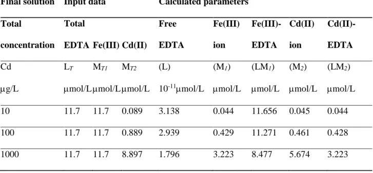
Table 1 shows parameters calculated using Eqs. (9)–(13) of the model of two 1:1 complex formations for constant concentrations of total EDTA ligand and total Fe(III) trace metal with various total Cd(II) concentrations. Total cadmium concentrations (101,000 g/L) introduced into the final solution corresponded to values of MT2 expressed in mol/L, as shown in Table 1.
Here Table 1
Initially, the free EDTA ligand concentrations were calculated using input data (corresponding values of LT, MT1, MT2, K1 and K2) and Eq. (9) of the model. The values (L) in Table 1 are extremely low, about 10-11 µmol/L, which are not comparable to those measurable in analytical practice.
Nevertheless, the accurate calculation of (L) is very important from the theoretical point of view, and because we used the predicted (L) values all other parameters could be obtained from the model.
Then, free Cd(II) ion concentrations were predicted using corresponding input data and Eq. (12), while the Cd(II)-EDTA complex was calculated from Eq. (11) as a difference between total Cd(II) and free Cd(II) ion (notice in Table 1 the values of (M2) and (LM2)). For dominant trace metal, first, the Fe(III)-EDTA complex concentrations were calculated from Eq. (10) showing mass balance relative to the total EDTA ligand (see (LM1) values in Table 1). Then, free Fe(III) ion concentrations were obtained from Eq. (12) as a difference between total Fe(III) and free Fe(III) ion, shown as (M1) values in Table 1.
From the results in Table 1, it is evident that by increasing the cadmium concentrations (100–1,000
g/L) in the final solution, the Cd(II) competed more efficiently with Fe(III) for complex formation with EDTA. The calculated concentrations (LM2) of the Cd(II)-EDTA complex and (M1) of the free Fe(III) ion are increasing. At the same time, the calculated concentrations (LM1) of the Fe(III)-EDTA complex decreased proportionally, which is altogether in line to mass balance relations shown in Eqs.
(11)–(12) of the model of two 1:1 complex formations. For example, if a total cadmium concentration of 100 g/L is introduced into the final solution (see Table 1), from the corresponding free Cd(II) ion concentration predicted by the model, we can estimate that about 52 g/L of free cadmium is bioavailable in culture. Therefore, from the predicted free Cd(II) ion concentrations for various total cadmium concentrations introduced into the final solution (shown in Table 1), we suggest that a total cadmium concentration in the range 1001,000 g/L is suitable for experiments. According to EPA, the cadmium concentrations in surface waters of impacted environments are often 2-3 µg/L or greater (EPA 2016).
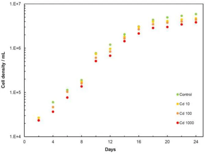
Cell growth and motility
Figure 1 shows growth curves of D. tertiolecta cells in cultures after the addition of cadmium of different concentrations. At a concentration of 1,000 g/L of cadmium, the cell density showed a maximal suppression that was only three times greater than the control sample, and therefore, the
corresponding concentration was selected for further experiments. Optical micrographs show some deterioration of cell shape, while flagellas are still present on the cell.
Here Fig. 1
Fluorescence images of cell culture in the presence of cadmium that show the presence of micrometre- sized particles possessing lipid characters are shown in Fig. 1SM (Supplementary material). We tracked the pathways and determined the speed of cell to analyse the effect of cadmium on cell motility. Figure 2SM shows representative D. tertiolecta cell pathways in control sample and in the presence of cadmium in the culture are shown on (Supplementary material). Around 65% of cells show the line type of pathways in control samples. For the first time we determined the speed of D.
tertiolecta cells, which corresponds to 74.29 6.13 m/s in the control sample. In contrast, in the presence of cadmium 91% of cells showed spot movement and 9% showed line type pathways that could correspond to a younger population of cells that had not been toxicated with cadmium yet. We determined that the speed of D. tertiolecta under the effect of cadmium corresponds to 50.26 3.38
m/s.
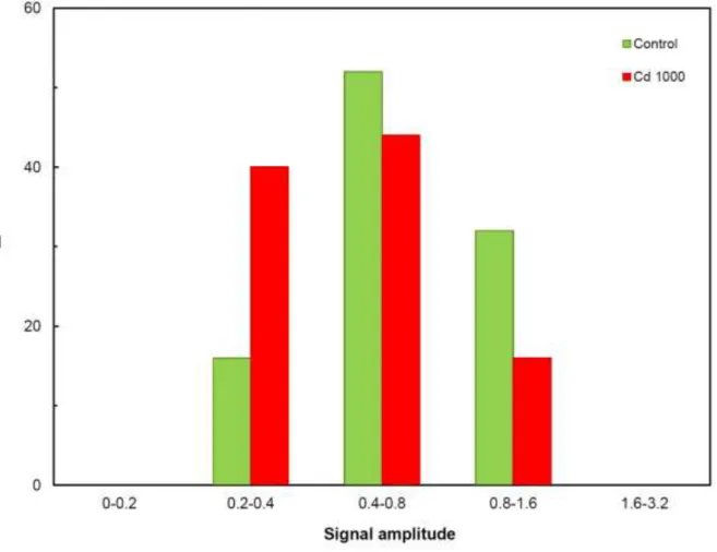
Amperometric characterization of D. tertiolecta cells
Amperometry at DME enabled us to detect interactions of single soft particles at the charged electrode (Svetličić et al. 2001). The amperometric signal appearance, shape and duration depended on the surface properties of the cell. Signal amplitudes reflected relative size distributions in suspension.
Figure 2 shows the frequency distribution of signal amplitudes in de-aerated cell suspension at the potential of -400 mV.
Here Fig. 2
The signal amplitude distribution was narrow and reflected monosuspension. In the presence of cadmium, the frequency of the smallest signal amplitude fraction increased, which probably corresponds to cell physiological activity manifested through released organic micrometre-sized particles that have surface-active characteristics.
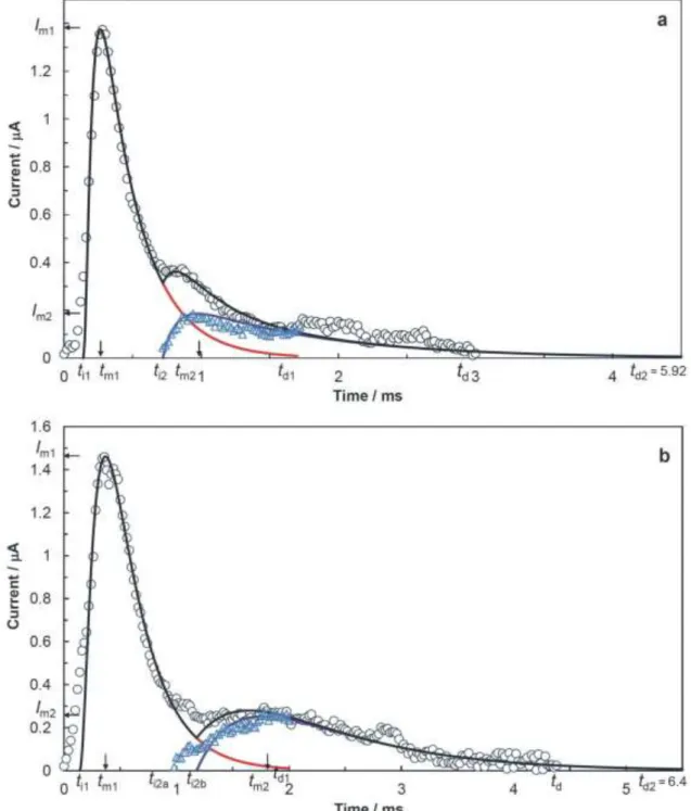
Kinetic interpretation of amperometric signals of D. tertiolecta cells
We applied the reaction kinetics model of the three step process and corresponding methodology to determine the kinetic parameters of adhesion and spreading processes from the amperometric signals of Dunaliella cells (Ivošević DeNardis et al. 2015; Ružić et al. 2010). Two amperometric signals of Dunaliella cells recorded in the stationary phase of growth at a potential of -400 mV are presented in Fig. 3 (open circles) for the control sample (a) and under the influence of 1,000 g/L cadmium as a stressor (b).
Here Fig. 3
To analyse the amperometric signal according to our methodology, first, it is essential to accurately determine the initial time and the time when the signal ends (i.e. when the current value decreases below 1% of current amplitude ). The amperometric signal of Dunaliella cell grown in control sample (see circles in Fig. 3a) had a current amplitude of 1.37 A at a of 0.28 ms and a signal duration is 3.0 ms. The amperometric signal of Dunaliella cell grown in medium under the influence of 1,000 g/L of cadmium as a stressor (see circles in Fig. 3b) is characterized with a current amplitude of 1.46 A at a of 0.36 ms and a signal duration of 4.36 ms. Using Eqs. (21)–(22), the calculated total displaced charges amount to 0.82 nC and 1.29 nC, while corresponding areas of the contact interfaces amount to 2.16 × 10⁴ m2 and 3.39 × 10⁴ m2, respectively. In addition, we estimated a volume of V = 114 m3 of the control Dunaliella cell by combining the contact area
ti td
Im
Im tm
td
Im tm td
qD
Ac
of the interface Ac, with the thickness of the final organic layer formed at the interface (d = 5.3 nm, (Ivošević DeNardis et al. 2015)). The volume of Dunaliella cell under the influence of cadmium as a stressor was estimated and the calculated value was 180 m3 (about 58% higher than the volume of control Dunaliella cell).
Further, according to our methodology, each of the amperometric signals was divided into a primary adhesion part and a secondary so-called bell-shaped part of the signal and then a separate analysis for each part was performed. A comparison of the determined kinetic parameters from amperometric signals using a reaction kinetics model for the primary adhesion parts and empirical fitting for the secondary signal parts is presented in Table 2.
Here Table 2
For the primary adhesion parts of the amperometric signals, the reconstructed current transients (red curves in Fig. 3) were obtained using the corresponding kinetic parameters ( , , and shown in Table 2) that were determined from the reaction kinetics model and Eq. (20). For both amperometric signals of Dunaliella cells the values of the rate determinng time constant τ2 are comparable. Time constants that are intermediate τ1 = 0.09 ms and fast τ0 = 0.05 ms for the first adhesion part of signal of Dunaliella cell under the influence of cadmium concentration of 1,000 g/L are two times slower than for the control signal of Dunaliella cell (see Table 2). The reconstructed current transients for the primary parts of the signals start at times ti1, had current amplitudes at times and end at times t > td1 (see red curves in Fig. 3).
The secondary parts of the signals, appearing at times t > ti2 (see Fig. 3a) andt > ti2a (see Fig. 3b), could not be described by the reaction kinetics model, although they both contain a significant amount of displaced charge (one third of the total displaced charge , shown in Table 2). Therefore, a further analysis was performed to obtain additional data (blue triangles in Fig. 3) relating to the secondary parts of the signals.
0 1 2 Q1
Im1
tm1
qD
For the signal data of Dunaliella cell in the control sample, additional data (blue triangles in Fig. 3a) at times t > ti2 (0.72 ms) was obtained as a difference between the signal data (o) and reconstructed current transient (red curve). Then, the corresponding data set was empirically fitted with two exponential functions of time (see blue curve in Fig. 3a) using determined time constants (fast f = 0.1 ms, slow s = 1.0 ms). The fast time constant f for the secondary part of signal of Dunaliella cell under the influence of cadmium in a concentration of 1,000 g/L was four times slower than for the control signal of Dunaliella cell (see Table 2). We obtained an amount of displaced charge of 0.24 nC, which is about half of and one third of as shown in Table 2.
For the signal data of Dunaliella cell under the influence of cadmium, the difference between the signal data (o) and the reconstructed current transient (red curve) was used to obtain additional data (blue triangles in Fig. 3b) for further analysis at times t > ti2a (0.98 ms). At times t > ti2b (1.18 ms), this obtained data set was successfully empirically fitted with two exponential functions of time (see blue curve in Fig. 3b) using f = 0.42 ms and s = 0.88 ms. The corresponding displaced charge is 0.44 nC (about half of and one third of , shown in Table 2).
These secondary signal parts of Dunalliela cells can be associated with the release of intracellular content during the spreading of organic film at the interface to its maximal extent. We observed that at the time interval ti2a < t < ti2b, 1.2% of the total displaced charge was not accounted for by the reaction kinetics model or empirical fitting (see Fig. 3b). This intermediate displaced charge could be prescribed to some transition process associated with the initial release of intracellular content.
The time constants obtained from the secondary parts of the signals (f and s) are significantly slower than adhesion time constants of the primary parts (see Table 2), which could be associated with the (i) attenuated effect of potential at the modified interface and (ii) stronger intermolecular interaction and reorganization of molecules in the film (Ivošević DeNardis et al. 2015).
Finally, a comparison of amperometric signals of Dunaliella cells recorded in the control sample and in the presence of cadmium (circles) with the overall best-fit curves of the signals (black curves) as a
Q2
Q1 qD
Q2
Q1 qD
qD
sum of (i) reconstructed current transients (red curves) of the primary parts obtained from the model and (ii) empirical fits of the secondary signals parts (blue curves) is shown in Fig. 3.
Agreement between the experimental signal data and the predicted data (using the sums of individual curves of the primary parts and the secondary parts of the signals) is rather good. Deviations of the total calculated displaced charges (Qtot = Q1 + Q2) from the experimental values (qD) are between 3.7% and 3.9%. Generally, since the corresponding deviation is small, a separate analysis of the primary parts of the signals from that of the secondary parts is justified.
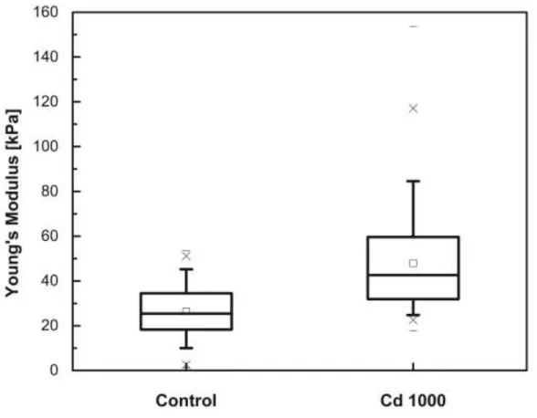
Nanomehanical characterization of D. tertiolecta cells
The elasticity of algae was measured in control samples and in samples with cadmium concentrations of 1,000 g/L. Compared to a purely elastic, very stiff material, D. tertiolecta shows a complex response to indentation, which can be seen as the appearance of multiple slopes in the force curves.
For both samples, 50 cells were measured and 20 force curves were taken and analysed for each cell.
Data were pre-processed using the JPKSPM software, and fitting as well as statistical analysis was performed using OriginPro 9 (OriginLab Corporation) and R as a free software environment. Outliers were removed after statistical testing (Grubbs test). We evaluated the significance of value differences using a one-way ANOVA with a significance level of 0.05 (p < 0.05 indicated as “*”, p < 0.01 as
“**” and p < 0.001 as “***”). As can be seen in Fig. 4, a distinct stiffening of the cells was observed by comparing only the initial slope of the retracted segments of the force curves.
Here Fig. 4
Young’s Modulus (YM) of the cells was calculated for the first 200 nm of the retracted curve (see Fig. 3SM in Supplementary material). For the algal cells in the control sample, the YM mean was 26.4 ± 0.4 and the median was 25.4 kPa. In the sample with a cadmium concentration of 1,000 g/L, the YM of the cells increased with a mean of 47.9 ± 0.8 kPa and a median 42.6 kPa. The YM of the
cells in the control sample was normally distributed while in the presence of cadmium it did not show a perfect normal distribution. The mean value shows a statistically significant difference (p < 0.001, analysed by one-way ANOVA), indicating an increase of stiffness of around 80%. For the cells in the presence of cadmium, a skewness of the value distribution was determined which could best be described using a log normal distribution.
Autofluorescence characterization of D. teriolecta cells
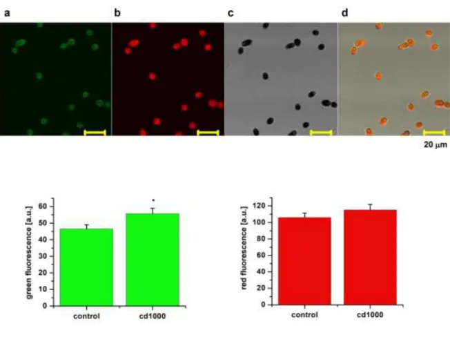
Employing laser scanning confocal fluorescence microscopy with an excitation at 450 nm, two emission windows were chosen based on spectrometric measurements (not shown), first in the green spectral region at 480–520 nm (Fig. 5 top a), and second in the red spectral region at 620–680 nm (Fig. 5 top b). The transmission mode (Fig. 5 top c) was used to evaluate the contour of the cell and the overall surface. In the control sample, the contour was evaluated to 24.5 ± 0.7 µm (n = 152 cells) and remained unchanged at 24.4 ± 0.4 µm in 1,000 g/L of cadmium (n = 109 cells). Surface area, which reached 53.8 ± 2.7 µm2 in control (n = 152 cells), remained unchanged at 55.2 ± 2.0 µm2 in the presence of 1,000 g/L of cadmium (n = 109 cells). The data confirmed recordable autofluorescence in both spectral channels.
Here Fig. 5
Intensity in the red spectral region was several times higher than that in the green region, as is expected for the major contribution of chlorophylls (Teplicky et al. 2017). When the intensity of the fluorescence recorded in the green and red spectral channels was compared among groups in the presence of 1,000 g/L of cadmium, we observed no significant change in the red fluorescence intensity (Fig. 5 bottom right). At the same time, we recorded a significant increase in the green fluorescence (Fig. 5 bottom left) in cells grown in the presence of 1,000 g/L of cadmium. Time- resolved imaging enables evaluation of the sensitivity of the endogenous fluorophores to their
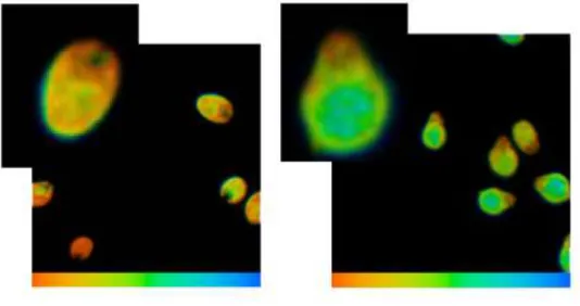
environment (Chorvatova and Chorvat 2014) and thus produces information that is potentially very useful for the examination of changes in the algae’s responsiveness to stress conditions. Fluorescence lifetime microscopy (FLIM) images were recorded using time correlated single photon counting following excitation at 475 nm. Algae fluorescence presented at least double exponential decays of 500 and 700 ps, as represented in the left side of Fig. 6.
Here Fig. 6
Note the slightly longer lifetime inside the algae when compared to the cell membrane area. Time- resolved images showed a longer fluorescence lifetime inside the cell body in the presence of 1,000
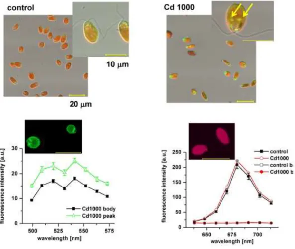
g/L of cadmium. Interestingly, we also noted deposits strongly fluorescing in green in cells in the presence of cadmium (Fig. 7 top right, arrows).
Here Fig. 7
To better understand the possible provenance of the deposits with increased emissions of green fluorescence in 1,000 g/L of cadmium (Fig. 7 top), we performed additional experiments. The deposits, which were mostly situated in the flagella region, exhibited a dark colour in reflection (data not shown). To establish spectra of this fluorescence, we separated recorded images based on the individual wavelengths of emitted light. We were able to record spectrally resolved images in the green spectral region between 499–573 nm, excited at 450 nm (Fig. 7 bottom left). These data, which were recorded with high sensitivity, uncovered weak but sustained autofluorescence in this spectral region with the most pronounced peak at 520–540 nm. When compared to the surrounding cell body, the fluorescence of the deposits also peaked at 520–540 nm but its values were significantly higher than in the body region. In addition, spectrally resolved images in the red spectral region, recorded between 640–713 nm (Fig. 7 bottom right), confirmed a maximum fluorescence emission at 680 nm, as expected for the peak of chlorophyll fluorescence. Spectra showed no change in 1,000 g/L of
cadmium. It is also noteworthy that FLIM images uncovered shorter fluorescence lifetimes (close to 500 ns) in 1,000 g/L of cadmium (Fig. 6 right) in this region of the cell when compared to the surrounding cell body. Interestingly, in the same region the fluorescence was practically missing in the control sample.
Protein expression profile
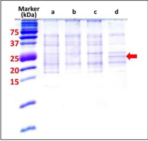
To examine protein expression in D. tertiolecta cells in the presence of Cd(II) ions, we applied sodium dodecyl sulphate polyacrylamide gel electrophoresis (SDS-PAGE). By means of this technique we separated and detected the proteins expressed in the algal cells. Several cultures of cells were set up and applied in this experiment as shown in Fig. 8.
Here Fig. 8
There were no released proteins in detectable amounts in the culture broth (data not shown), but it should be noted that these were very dilute solutions. The total protein fraction showed a crowded picture for each sample that was difficult to analyse in detail. The SDS PAGE result with the soluble protein fraction showed that mostly all the proteins can be detected in each sample independent of the various conditions applied. However, there are some differences between the protein expression profile of the Dunaliella cells grown in the seawater and those grown in the presence of toxic Cd(II) ions. A protein band close to the 25 kDa size marker band gradually increased the relative intensity (compared to its neighbouring band intensities) as the stressor concentration increased. This band is denoted by the arrow in Fig. 8.
The protein(s) expressed under stress conditions related to the SDS PAGE band in question were identified by mass spectrometry using a peptide mass fingerprint analysis. According to this identification method, the search in the Uniprot database supplemented by the green plant sequences suggested similarity with the proteins depicted in Table 3.
Here Table 3
All of the significant hits belong to D. salina, an organism that is related to D. tertiolecta. Thus, the additional band around 25 kDa in lane d (Fig. 8.) could contain a chlorophyll a-b binding protein. The alignment shown below the chlorophyll a-b binding protein of LHCII type I, is chloroplastic between the two algae and using the CLUSTAL O (1.2.4) multiple sequence alignment routine yielded ~ 60%
sequence identity (see Table 1SM in Supplementary material). This confirms that the protein identified in the above experiment is indeed a chlorophyll a-b binding protein of the D. tertiolecta.
Discussion
We applied a new methodology based on a generalized mathematical model to predict the concentration of free cadmium in culture. Model calculations enabled us to create experimental conditions that are harmful for cells in culture. We selected a maximal cadmium concentration of 1,000 g/L, which corresponds to 600 g/L of free cadmium that refers to the bioavailable fraction.
We examined algal cells’ responses to laboratory-induced cadmium stress, focusing on the biointerface and intracellular changes by employing a multimethod approach. The biointerface is characterized in terms of surface properties (cell stiffness) and adhesion dynamics on a single cell level. The intracellular response was examined in terms of the cells’ autonomous features (i.e. motility and autofluorescence) and protein expression obtained from the cell culture. The results show that in spite of very a high cadmium concentration and prolonged cell exposure, the cells grew without significant suppression of growth dynamics. An increase in physiological activity was manifested through relased lipid surface-active microparticles in culture. Different cell motility and pathway types were observed, which provides insight into cell viability. Cells showed slower motility and vibrating at the spot when cadmium is present in the culture. The difference in adhesion behaviour was determined to be two times slower for initial attachment and deformation, while rate-limiting
steps referring to the spreading of released intracellular content are not significantly different in comparison with the control. AFM measurements revealed that cells are significantly stiffer in the presence of cadmium, which influenced the dynamics of the initial contact of the cell at the interface.
The YM of D. tertiolecta cells in the control sample agree with an independently conducted study (unpublished data, F. Pillet et al.). Pillet et.al. developed a protocol to attach motile cells to the mica substrate to image them. They reported that cell surface properties (stiffness and hydrophobicity) change with age and those data support well-determined adhesion dynamics of cells at the interface.
There are few reports in the literature about structural and mechanical characterization of other algal cells such as diatoms (Hildebrand et. al. 2008; Pletikapić et. al. 2012), which appeared to be much stiffer (YM is higher about three orders of magnitude) due to the silica cell wall.
Also, we recorded the fluorescence emission of Dunaliella algae in two spectral regions (green and red) and, for the first time, we demonstrated the possibility of recording time-resolved fluorescence directly in living cells. In the presence of cadmium in the culture, the red fluorescence emission attributed to chlorophyll was unchanged. Such a cell response could be accompanied by embedding the waste into vacuoles (probably carotenoids), which was detected as increased emission in the green spectral region mostly around the flagella. Wan and Zhang, 2012 reported that the presence of green fluorescent deposits suggests the effect of Cd(II) on vesicular trafficking and/or transport of Cd(II) into vacuoles. Accumulation of the green fluorescence in these deposits may result from the production of beta-carotenes as already described in the algae under a stressor (Shariati and Yahyaabadi 2006; Belghith et al. 2015). Thus, the appearance of deposits in the green spectral region could be attributed to chloroplast-related pigments of the photosystem, such as carotenoids, and/or to oxidative metabolic changes. Beta-carotenes were proposed to prevent cell damage following exposure to Cd(II), possibly as a result of antioxidant responses (Pinto et al. 2003) and/or prevention against free oxidative radicals (Shariati and Yahyaabadi, 2006).
There is controversy in the literature about chlorophyll and carotenoid contents under stress conditions. For instance, an elevated Cu(II) concentration increased the chlorophyll and carotenoid content in Dunaliella cells (Miazek et al. 2015; Nikookar et al. 2005), while Hg(II) pollution
decreased the chlorophyll a content (Zamani et al. 2009). Only few studies have been conducted on the effect of stressors on protein expression. Dunaliella tertiolecta cells cultured in the presence of 5, 10, 20 and 50 µM HgCl2 showed enhanced expression of two proteins of about 29 and 38 kDa, but the proteins were not identified in that study (Zamani et al. 2009). Here we observed the appearance of increased amounts of a protein of similar size. This protein showed differential expression under normal and Cd(II) stressed conditions and was identified by the peptide mass fingerprint assay as a chlorophyll binding protein of Dunaliella salina (Fig. 8 and Table 3). There is limited information about the genome of Dunaliella tertiolecta, but we could assign this hit to this species by searching for similar sequences in protein databases (Table S1). The identified protein is related to chlorophyll homeostasis in the light-harvesting complex (LaRoche et al. 1990). It binds at least 14 chlorophylls (8 Chl-a and 6 Chl-b) and carotenoids such as lutein and neoxanthin. In a water-soluble form it may perform temporary storage and carry chlorophyll (Damaraju et al. 2011). Therefore, it may play a role in the energy production needed for the defence mechanism and/or in the protection against the heavy metal stressor. The fact that the red fluorescence was maintained even at the high Cd(II) concentration applied in our study may be related to the above functions.
It is worth mentioning that carbonic anhydrase (CA) is also included among the hits in Table 3, although it has much higher molecular weight than the area covered by the band investigated. The reason for this could be that we detected one of the two major CA domains (258 and 265 amino acids long) in our experiment. The Zn(II) ion in the CA active centre is easily exchanged to Cd(II). CA has even been identified as a Cd(II) enzyme in marine diatoms (Lane et al. 2005). In Mytilus galloprovincialis the involvement of CA in the response to cadmium exposure was suggested by Caricato et al. (2018). As this enzyme can supply ribulose 1,5 biphosphate carboxylase with carbon dioxide to fix in the photosynthetic pathway, it may be a part of the defence system in the algal cells as well.
Conclusion
Algal cells of D. tertiolecta showed successful adaptation to toxic cadmium concentrations in culture.
The cells adapted to a new life strategy through cell shape deterioration, slower motility and an increase of physiological activity. No significant suppression in growth dynamics shows how the cell fights back by increasing the active surface area against toxic cadmium in the culture. There was no change in the endogenous fluorescence in the red region (associated with chlorophyll) but there was a change in the green region (possibly associated with cadmium vesicular transport and beta carotene production), which provides insight into the cells’ adaptation strategy to maintain photosynthesis.
Specific responses of natural fluorescence of cells under the influence of cadmium are most likely associated with the identified chlorophyll a-b binding protein. It seems that another identified protein, carbonic anhydrase, plays an important role in the photosynthetic pathway. Since production of these proteins can be related to the maintenance of the photosynthesis representing one of the cell defence mechanisms (Kim et al. 2005), it may also indicate the presence of toxic metal in seawater. The expression of proteins may affect the cell surface’s properties and therefore the dynamics of cell adhesion at the interface. Cells behave stiffer under stress with cadmium, and thus the initial attachment and deformation of cells is slower at the interface. This multimethod approach enabled us to better understand cell responses under laboratory-induced cadmium stress to predict the fate of algae in a marine environment. Our results will substantially contribute to the biophysics of algal cells on a fundamental level.
Acknowledgments
This work was conducted and supported by project Algal cell biophysical properties as markers for environmental stress in aquatic systems (ID 21720055) funded through the International Visegrad Fund. AMH acknowledges support from the Integrated Initiative of European Laser Infrastructures LASERLAB-EUROPE IV (H2020 grant agreement no. 654148). AW acknowledges funding from the Austrian Science Fund (project number P29562N28). We would like to thank (i) Tarzan Legović for discussing cell motility analysis with us, (ii) Jagoba Iturri and José Luis Toca-Herrera for
discussing cell nanomechanics with AW and (iii) project partner Josef Sepitka for his participation and interest in this work. The authors acknowledge networking effort within COST Action CA15126 ARBRE MOBIEU.